
Introduction to Monte Carlo concepts & basic techniques -
Shot noise & thermal noise
ECE generic - segment 1
1. Introduction: a simple problem
First, a description of the background.
https://www.youtube.com/watch?v=Sh1ZeWhAtRI
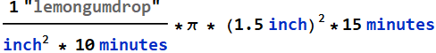
Let’s assume that all the raindrops were lemondrops and gumdrops, and the kids all stood outside with mouths open wide. Assume that all the kids have mouth of the same size, which is:
![]()
![]()
or 7 ![]() . Let the lemon/gumdrops density is
. Let the lemon/gumdrops density is ![]() per 10 minutes. If we have 100 kids all stand outside with mouth open wide for 15 minutes, how many lemon or gumdrops would each kid catch? (Think about what right questions are - Asking the right questions is 80% of the work). How to solve this problem?
per 10 minutes. If we have 100 kids all stand outside with mouth open wide for 15 minutes, how many lemon or gumdrops would each kid catch? (Think about what right questions are - Asking the right questions is 80% of the work). How to solve this problem?
1.1 Discussion
First, we can think of the average of lemon/gum drops that each kid can get. The average is easy to calculate:
![]()
But does that mean every kid would get exactly 10.6 lemon/gumdrops? If we count the number of “raindrops” each kids get, and tabulate on a histogram, do they all get 10, 11? or would some get 5, other would get 15 etc... Is it possible for some to get 20?
How do you answer the questions above. Or could it be that it doesn’t have an answer? If you have several groups of 10,000 kids each, for example. Would there be a common pattern, or some unique shape in all of their histograms? Or will the histograms be totally random and completely different from each other?
In the follow, you should follow the guidelines to gain an understanding and see if you can answer those questions at the end.
One way to study this problem is the Monte Carlo method:

1.2 Computer simulation
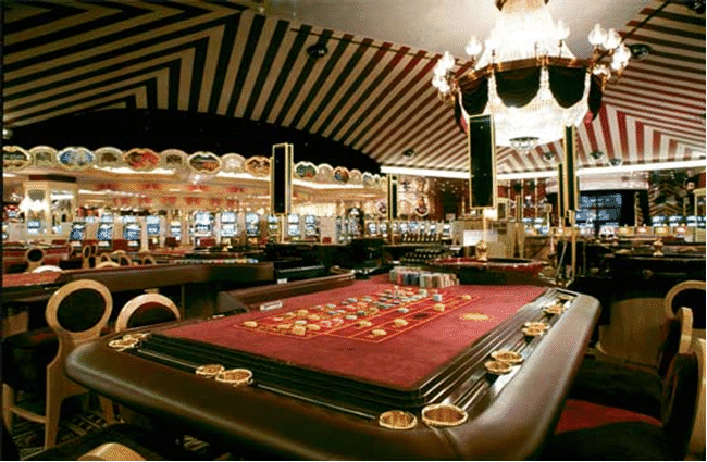
We can use the computer to simulate 100 kids’ mouths and rain drops.
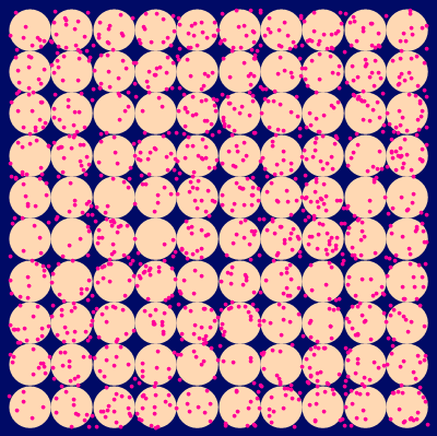
Here are the mouths:
 |
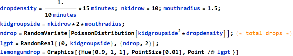
The left handside is the model of the right handside that is easier for counting (lest the right hand side swallow lemon/gumdrops before we finish counting). Next, let’s make lemongumdrops:
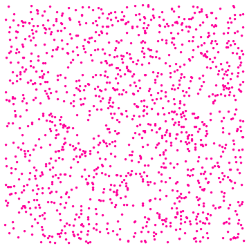
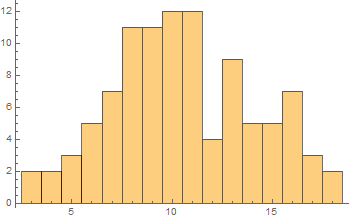
Now, let’s see who catch what by putting mouths and lemongum raindrops together:
![]()

We will count for each mouth:
 |
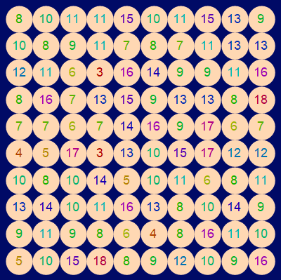 |
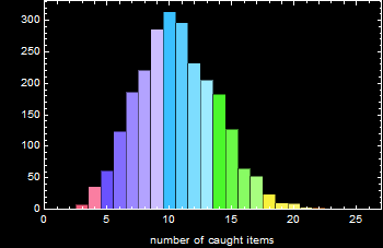
There we have it. Lucky kids could get 18, 19 or more. Less lucky ones got 5 or less. Let’s check the histogram
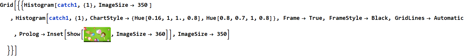
|
|
We see that the lucky ones could catch several times more than the unlucky ones. The mean is:
![]()
![]()
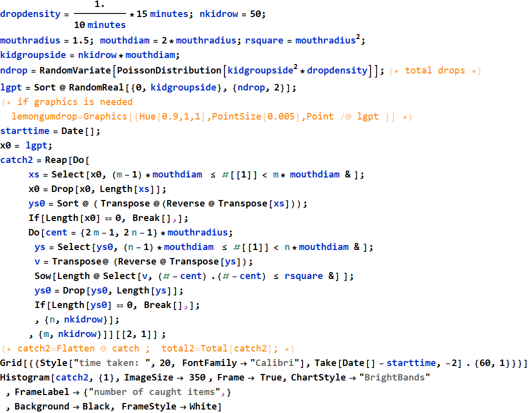
To improve statistics, we can run the simulation with larger sampling populations. The code below is for 2500 kids (use your discretion to decrease the size if the computer takes too long). Based on your result, find:
- what is the chance for a kid to get only 4 candies? (of course, under the same condition: ![]() per 10 minutes and the kid stands for 15 minutes).
per 10 minutes and the kid stands for 15 minutes).
- what is the chance to get exactly 10? (many think it is about 50%-50% and that is very wrong).
- what is the chance to get 15 and 20, respectively
- show your histogram(s).
Here is the code for 2500 kids (50 by 50). (Written a little longer than the above for faster execution. On slower computers, reduce nkidrow to 30 or 25, for example)
1.3 Computer simulation - higher sample polulation
2. Poisson distribution
2.1 Discussion
As one can see from 1.2 and 1.3 above, the distribution is quite consistent as we run the code several times. In fact, it has a name: Poisson distribution.
You can read up an interesting application during WW2 when the British tried to determine if German V-1 and V-2 bombers were sufficiently accurate navigationally, to target high-value facilities: https://www.britannica.com/topic/Poisson-distribution
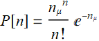
For a given mean value ![]() (such as the expected average of the candies per kid), the probability for n candies is:
(such as the expected average of the candies per kid), the probability for n candies is:
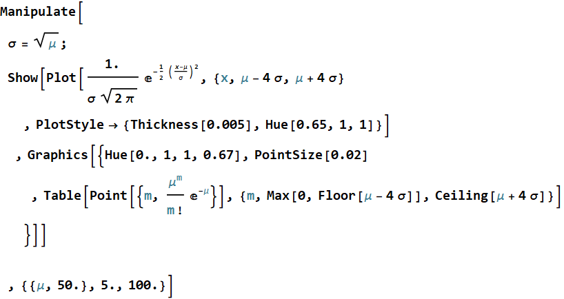
2.2 Demo 1: using Mathematica built-in Poisson distribution function
Below is a demo that uses built-in Poisson distribution of Mathematica. You can see the distribution reaches certain shape as n-> 10,000.
code
2.3 Exercise/demo: 1-dimension uniform random distribution
Exercise
Generate 5000 RandomReal betweet 0 and 1, sort them into 1000 bins, from [0-0.001), [0.001-0.002),...[0.999-1). Count the number in each bin and make a histogram
Answer
2.4 Asymptotic approximation for large mean
In practice, when mean ![]() is large, such as >50, Poisson distribution can be conveniently approximated with a Gaussian:
is large, such as >50, Poisson distribution can be conveniently approximated with a Gaussian:
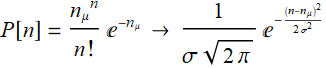 where
where ![]()
3. Electrical current: Drude model
3.1 Review: Drude model of electron transport
Consider the Drude model below for electrical conduction:
3.2 Poisson fluctuation
In the app above, if we count the number of electrons crossing a point per a given time interval Δt, will we obtain exactly the same # of electrons everytime? Clearly, we won’t. The number of electrons per time interval will fluctuate. For simplicity, we’ll treat all electrons as having the same drift velocity. Then we have the demo below
code
4. Shot noise
4.1 Discussion
As illustrated in 3.2, the number-of-electrons fluctuation per measurement interval Δt means current fluctuation.
4.2 Current shot noise app
4.3 Dark current of detector: an example
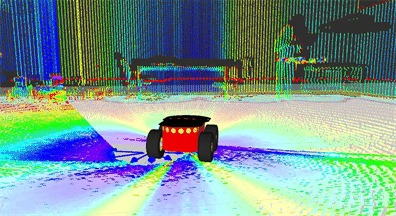
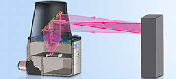
Suppose we have a robot that uses a lidar to probe its surrounding. It sends out laser pulses with 1-ns duration. It has a receiver (optical detector) with a responsivity of 0.5 A/W, with a dark current of 1 mA. (0.5-A/W responsivity means that for every watt of optical power incidents on it, it yields 0.5-A current; and 1-mA dark current means that even without any light, i. e. zero optical power, it still yields a steady current of 1 mA).
Calculate the number of electrons of dark current during one laser pulse.
Hint: use this formula: 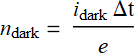
Answer
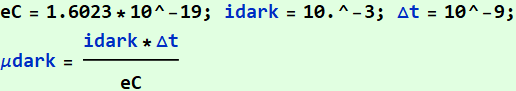
![]()
4.4 Lidar signal current
The laser backscattered power on the detector is 0.5 μW. Multiply this with the responsivity to get signal current. Then, calculate the number of signal electrons for one laser pulse. (Use the same formula above, but ![]() instead of
instead of ![]() ).
).
Answer
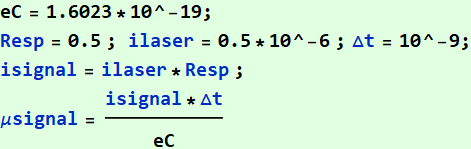
![]()
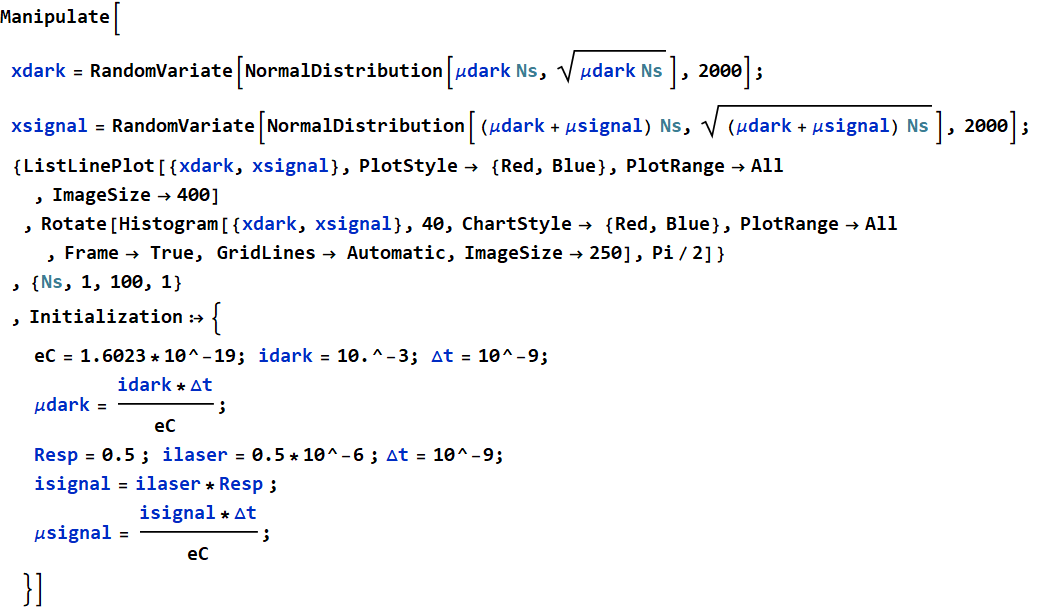
4.5 Simulation
The total electrons = lidar signal electrons + dark current electrons.
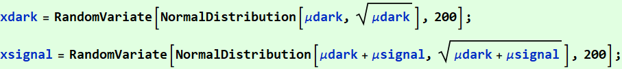
- generate xdark=200 samples of dark current electrons, using Gaussian approximation of Poisson’s distribution, which is: 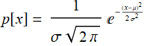 where μ is the average # of dark electrons and
 ![]() .
.
- generate xsignal=200 samples of total electrons that include both dark and lidar electrons, using the same formula but with μ being the average of total electrons.
- ListLinePlot both in the same plot. Discuss if you can see any difference between them (which is the lidar current).
Answer
![]()
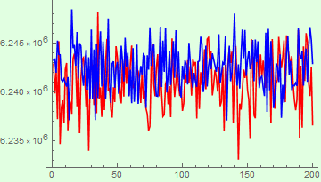
Discussion: It is clear that the signal is too small compared with the noise and it is hard to see any difference.
4.6 Signal accumulation
Instead of measuring with just one pulse, we can accumulate many pulses. Use the same code above, but allow Ns, the number of pulses, be “Manipulatable”. Vary Ns from 1 to 100 and discuss what you find.
Plot a histogram for each of these two cases:
1- data of dark electrons # and total electrons # with 1 pulses. (histogram of xdark and xsignal in the same plot, each with different color, use the 200 pts you generate above.)
2- same as above with accumulated data with 100 pulses.
Compare the SD of the two distributions for the two cases and discuss (remember the ![]() rule. When you increase the number of samples 100 times, the total increases linearly, but the SD increases only as the square root of it. If you take the average by dividing the mean by the number of samples, then the mean stays the same:
rule. When you increase the number of samples 100 times, the total increases linearly, but the SD increases only as the square root of it. If you take the average by dividing the mean by the number of samples, then the mean stays the same: 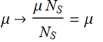 , but the
 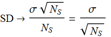 ).
).
Answer
5. Johnson noise: an example
5.1 Discussion
Note: use the APP on noise to gain a gut feeling about thermal noise.
Electrons in a medium above absolute-zero temperature do not rest, but agitate randomly (quantum mechanically). Thus, there is a fluctuating current, of which the average is zero, but not the mean square. The kinetic energy of electrons ~ ![]() . The noise power is:
. The noise power is:
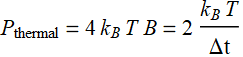
where ![]() is the Boltzmann’s constant and B is the measurement bandwidth, which is
is the Boltzmann’s constant and B is the measurement bandwidth, which is ![]() if we think in terms of sampling duration. If the curcuit resistor is R, then:
if we think in terms of sampling duration. If the curcuit resistor is R, then:
![]()
Or: 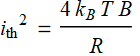 ;
; 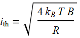
In terms of voltage, 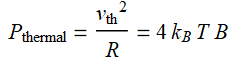 ;
; ![]()
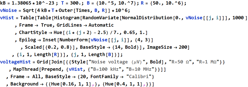
![]() =1.38065×10^-23 Joule/Kelvin; and for future reference, electron charge =1.6023*10^-19 C.
=1.38065×10^-23 Joule/Kelvin; and for future reference, electron charge =1.6023*10^-19 C.
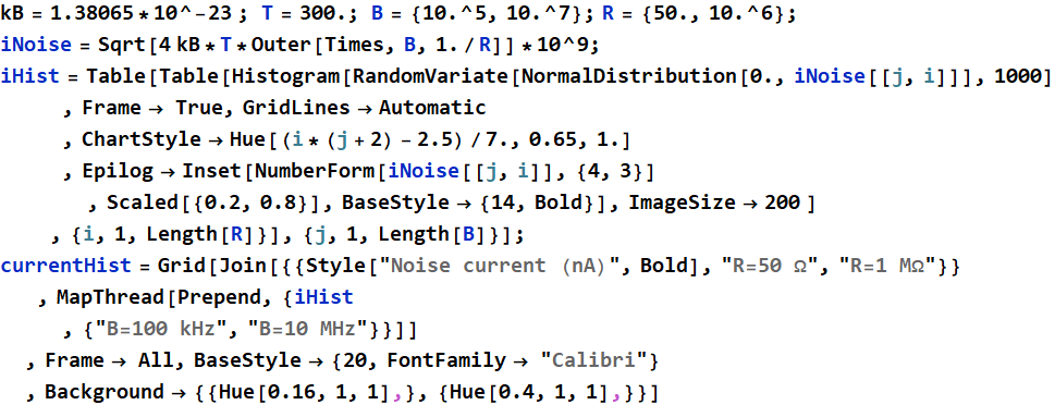
5.2 Johnson noise: an exercise
Write a computer program to calculate the current noise and voltage noise at least 4 cases: bandwidth B= 100 kHz and 10 MHZ; impedance R 50 Ohm and 1 MOhm. Let T=300 K. (2 cases of BW x 2 cases impedance = 4 combinations).
Answer

| Noise current (nA) | R=50 Ω | R=1 MΩ |
| B=100 kHz | 5.75635 | 0.0407036 |
| B=10 MHz | 57.5635 | 0.407036 |

| Noise voltage (μV) | R=50 Ω | R=1 MΩ |
| B=100 kHz | 0.287818 | 40.7036 |
| B=10 MHz | 2.87818 | 407.036 |
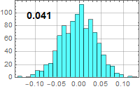
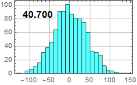
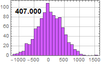
5.3 Simulation
Use your results in 4.1 to simulate 1000 voltage measurements for the 4 cases above and plot histograms. Compare your histogram with those shown in the APP side by side.
Answer
| Noise current (nA) | R=50 Ω | R=1 MΩ |
| B=100 kHz | 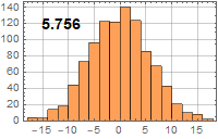
|
 |
| B=10 MHz | 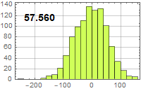
|
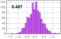 |
| Noise voltage (μV) | R=50 Ω | R=1 MΩ |
| B=100 kHz | 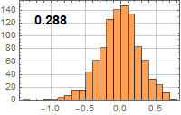
|
 |
| B=10 MHz | 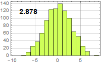
|
 |
5.4 An example with op-amp
Suppose you have the following simple amplifier (T=300 K)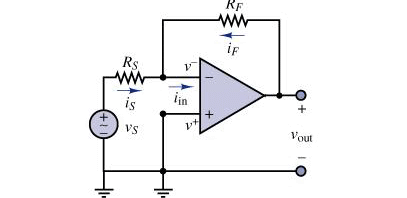
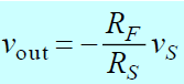
Let ![]() ,
, ![]() , What do you expect the noise level on the output for bandwidth = 1 MHz.
, What do you expect the noise level on the output for bandwidth = 1 MHz.
Answer
The noise of the output is a sum of the input noise and the thermal noise of the feedback resistor itself, ![]() .
.
Hence: 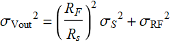
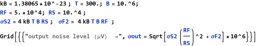
| output noise level (μV) = | 70.5006 |