Introduction to Monte Carlo concepts & basic techniques -
Common distributions
ECE generic - segment 2
1. Introduction: Some basic stochastics concepts reviewed
1.1 Uniform distribution
Ask a physicist or engineer to make 20 points uniformly on a line, this is what he/she will make:

Ask a statistician 20 uniform points on a line, this is what he/she will make:

Both have to do with uniformity. One type of uniformity is exact and deterministic. The other is uniformity with randomness: the probability for a point to be anywhere on the line is uniform. But the event is random, also known as stochastic phenomenon, hence the points can end up anywhere.
In the previous lecture, we have done a Monte Carlo simulation of this:
The rain is uniform in the sense that any lemon/gumdrop has a uniform probability to fall into any mouth. But the actual final location - because of so many uncontrollable factors of random air movement, falling-object mechanical motion, Bernouilly air dynamics and air resistance, etc - is not uniform in the physics/engineering sense - which is essential for a stochastic phenomenon (otherwise, it wouldn’t be stochastic). So, we did use RandomReal to generate a two-dimensional random arrays with uniform distribution for the lemon/gumdrops. But did the kids have uniform chance to get any number of lemon/gumdrops? They get Poisson distribution as you have learned.
1.2 Non-uniform distribution
What is it like to have a NON-uniform distribution? Watch this, known as a Galton’s board (click on link)
You see that the candies (or color marbles) are NOT spatially uniformly distributed. The center has more than the two sides.
This is how it works: without those path-deflecting pegs, the balls would fall straight down the center. However, as a ball goes through each stage, it hits a peg and has EQUAL chance to go left or right. It is like flipping a coin. If it keeps on flipping head, it goes one side, for example, let’s say left and left until getting to the furthest left bin. Or tails and tails and ends up in the furthest right bin. But that’s rare to flip that many heads or tails in a row. Most have roughly equal chance to flip head or tail and end up somewhere in the middle. Hence, we have a non-uniform distribution.
2. Galton board simulation: Binomial distribution
2.1 Tutorial
It is extremely important for you to learn techniques of the Monte Carlo method: to simulate a random process using computer. Hence, you will start learning to simulate Galton’s board in this exercise. Follow instructions below, then do the work at the end. Later, when you learn about stochastic processes like Brownian motion-Wiener process for stochastic calculus, you will need all these stuffs.
To simulate a ball going left or right, we use:
![]()
![]()
But instead of 0 and 1, we can convert it to +1 and -1 to make it goes right or left equally (you will learn later something similar to this: random walk. Perhaps you might have read this book “A Random Walk Down Wall Street”). This is done with this:
![]()
![]()
To make the ball go through many stage, we do this:
![]()
Convert 0 and 1 into -1 and 1:
![]()
Which bin does the ball end up in? by adding up all the left (-1) and right (+1). Use function Total to get that.
![]()
![]()
The ball ends up in bin 4 in the left (if you run again, you will get a different number - that’s what’s random simulation is about). This is what you will do: generate 1000 balls like the one above, get their final bins, and make a histogram to find how many balls in each bin. Suggestion: you can use Table or Do loop to generate 1000 balls. This is an example to generate the paths of only 5 balls
To get the final bin position, we just have to do Total:
![]()
![]()
This means ball 1 is in left 8 bin, ball 2 in right 6 bin, ball 3 in left 2 bin, ball 4 in left 8 bin, and ball 5 in right 2 bin (if you run again, you will get a different number). When you do for a thousand balls, you don’t want to print out to see for sure, just use ; to terminate each statement. Show only the histogram. Is the distribution of balls spatially uniform?
result:
It looks like in those experiment demos on Youtube.
2.2 Galton board simulation
Exercise - Galton’s board with variable stages
If you feel you do well with simulation technique, do a simulation of the Galton board with input choice such as the number of stages and balls etc. See the simulation below to get an idea what it is about.
Answer
You don’t have to do the thing below if not feel up to the task. But you should look through as it gives you another perspective how a seemingly uniform random process leads to a non-uniform distribution. But if interested, you can try to see how far you can program demo like the one below: one can vary the number of stages, the number of balls, and simulate each ball falling path. You can vary the ball number and see the histogram fills up similarly to the physical bins in real experiments.
code
Note: this is also a preview of what we will learn later: imagine the ball as an investor on “a random walk down Wall Street”. Each stage it bounces is an investment decision. You can buy or sell and your porfolio increases (say, move to the right) or loses (move to the left). The ball path is a representation of a stochastic process path. What will be your porfolio as a function of time? This type of calculation is in the field of “stochastic calculus” that is the foundation of financial calculation that we will study later.
2.3 Binomial distribution
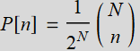
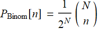
One can prove that the distribution of the balls of a Galton board is binomial distribution, expressed as:
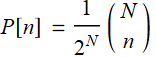 ; for n=0, 1, .., N (2.1)
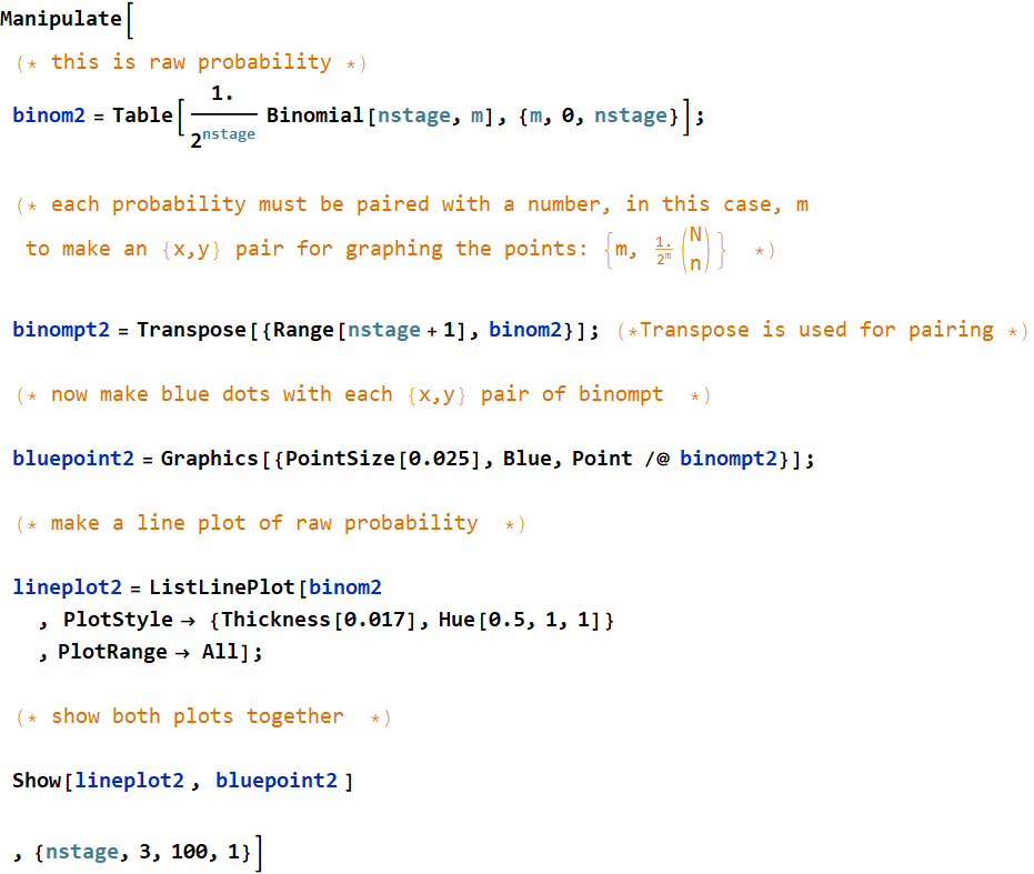
Exercise - plot the binomial distribution
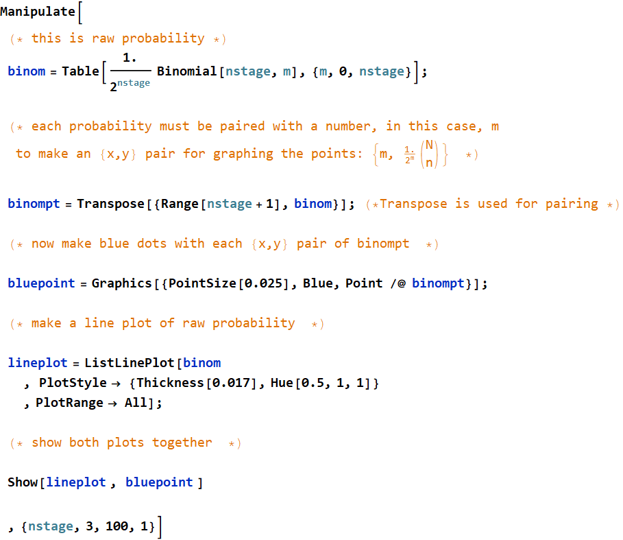
Make a Manipulate loop of plot of
 ; for n=0, 1, .., N (2.1)
where one can vary control variable N . (Do not use symbol N in Mathematica since it is a reserved named function). For example, for nstage=8:
![]()
Note that the total is always = 1
![]()
![]()
Answer
2.4 An example of binomial distribution: coin flipping
A more common example of binomial distribution is the game of coin flipping. Let’s consider this exercise
Exercise
We have 500 students playing the game of coin flipping. Assume the coin is perfectly fair, which means it has equal chance to flip head or tail. Everyone flips 12 times. Approximately many students can you expect to get:
1- 2 tails and 10 heads? (in any order, of course)
2- 3 tails and 9 heads?
3- 4 heads and 8 tails
4- 9 tails and 3 heads?
5- what is the chance for a student who can flip 12 heads in a row?
6- which of the question from 1-5 above you can answer with a previous calculation and there is no need for any new calculation?
7- How many students can you expect to get anywhere from 1 to 5 tails? Is is equal to the expected number of students who get from 1 to 5 heads?
Note: If you want to calculate the probability using the formula:
 ; for n=0, 1, .., N (R.2.1)
There are 2 ways, you can use Mathematica function BinomialDistribution, or just this (recommended to use it here):
![]()
If you want a floating point number instead of a fraction like above, use a decimal point (red dot below) on any number like this:
![]()
Answer
For questions 1-5:
![]()
![]()
We can put the answer in a table:
| outcome | probability | expected # of students |
| 2 tails 10 heads | 0.0161133 | 8.05664 |
| 3 tails 9 heads | 0.0537109 | 26.8555 |
| 4 heads 8 tails | 0.12085 | 60.4248 |
| 12 H/T in a row | 0.000244141 | 0.12207 |
6. which of the question from 1-5 above you can answer with a previous calculation and there is no need for any new calculation?
We don’t have to do question #4 because “9 tails and 3 heads” has the same chance as “3 tails and 9 heads”. The coin doesn’t care head or tail. Both has equal chance.
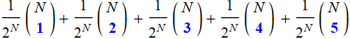
7. How many students can you expect to get anywhere from 1 to 5 tails? Is is equal to the expected number of students who get from 1 to 5 heads?
First, we can answer the second part. The expected number of students getting from 1 to 5 tails is the same as those with 1-5 heads for the same reason stated in answer 6 above.
To calculate the probability of 1-5 tails, we just have to add:
![]()
![]()
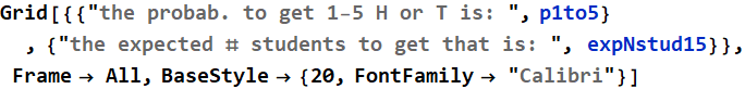
| the probab. to get 1-5 H or T is: | 0.386963 |
| the expected # students to get that is: | 193.481 |
It is more elegant if we use Total:
| the probab. to get 1-5 H or T is: | 0.386963 |
| the expected # students to get that is: | 193.481 |
3. Normal distribution as the limit of binomial distribution
3.1 Asymptotic behavior of binomial distribution with large stage number
In the last exercise, this is what you might have:
We will change the code above slightly: instead letting the x-axis to be {0,1,2,3,...nstage}, we will shift it by  to make:
It’s no big deal, the x-axis is only for plotting and it is prettier to make it symmetric across zero.
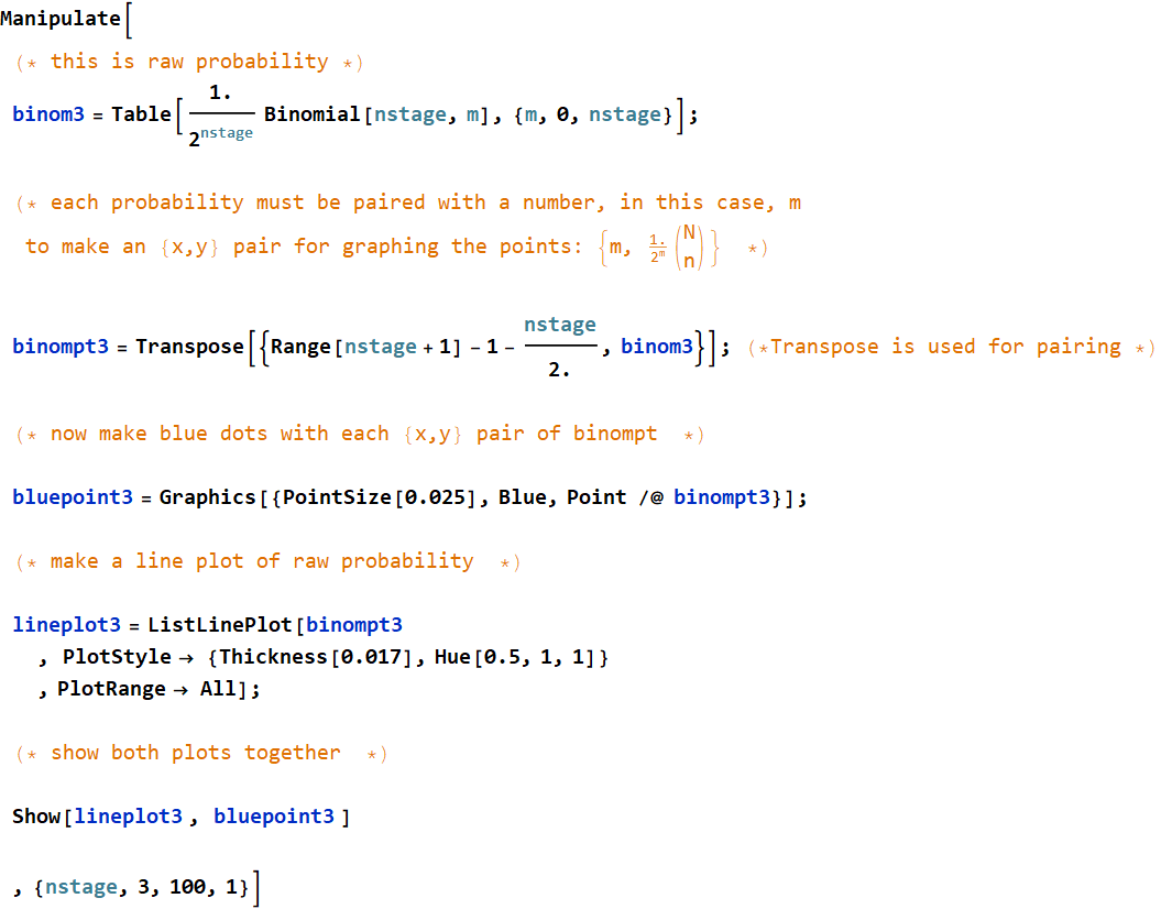
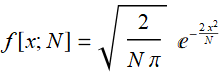
What do you think the curve would asymptotically approach to as nstage -> ∞? As nstage gets larger, the curve looks smoother and smoother. Can there be some mathematical function f[x] that approximate the binomial curve?
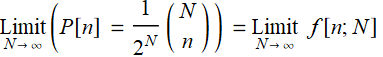
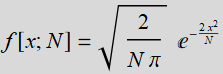
The answer is yes, and that function is:
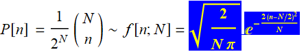 (R.3.1)
and
 (R.3.2)
we highlight the function because it is such an important function that we will encounter over and over throughout the course. Eqs. (R.3.1) and (R.3.2) say that as N gets ∞, the two functions at their limits become equal. This result is a consequence of a well-known theorem: central-limit theorem that explains why Gaussian or Normal distribution are found in so many phenomena.
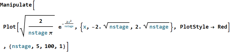
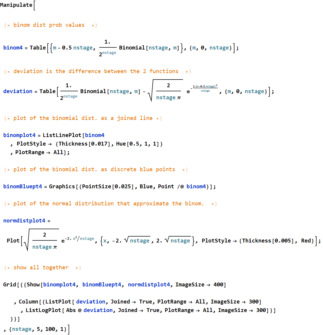
Exercise - demonstrate the approximation of binomial with normal distribution with graphics
Write a code showing (R.3.1). Plot the right hand side and the left handside of the equation (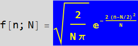 ) on top of each other, and show that at large nstage, they become practically equal.
You already have the code to plot 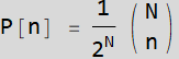 . However we’ll do one more thing: to make thing prettier with symmetry, we will shift the x-axis by
  . Hence the right handside function becomes:
 where
where 
You can use the code below for plotting  . You must combine both plots to show they are on top of each other.
You can take a sneak peek at the answer but should write your own code.
Answer
Exercise - comparing Poisson with normal distribution with graphics
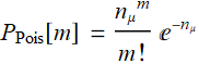
Do you recall this from Lesson 3:
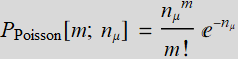 (R.3.3)
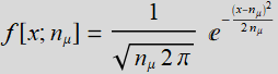
where ![]() is the mean or expected (or average) number of lemon/gumdrops each kid can get, and m is the actual number
is the mean or expected (or average) number of lemon/gumdrops each kid can get, and m is the actual number

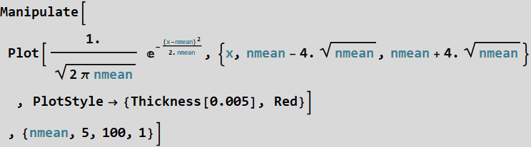
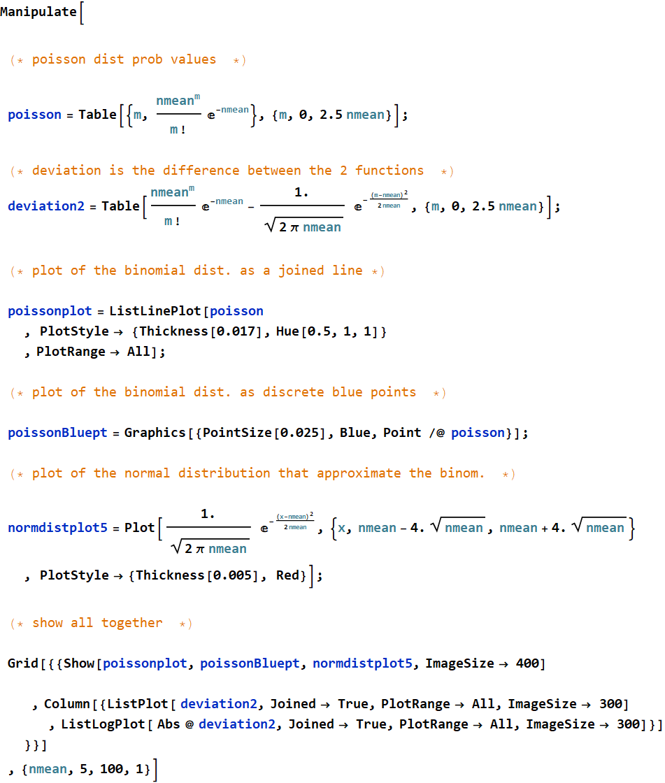
Compare this distribution by plotting it directly above this given form of normal distribution, similarly what we did above for binomial dist. vs. normal dist.
 (R.3.4)
You can use this code to plot the normal distribution:
Answer
3.2 An interpretation of normal distribution
What is the meaning of what we did above? When we measure or make an observation, the quantity we measure may fluctuate randomly because of uncontrolled effects. These random effects can make the value a bit higher or lower, like a ball on a Galton’s board may bounce to the left or right or left ... etc. Eventually, after so many bounces the ball is not always exactly and deterministically at the center as it should be but has a spread of possible values, which means a distribution.
In the large number of bounces limit, the distribution becomes what we call normal distribution:
 =>
=> 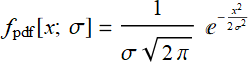
More generally the function f[x] doesnot have to center on zero. It can center on any value, which we will call μ:
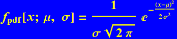 (R.3.5)
μ is called the mean, and σ is called standard of deviation. This is among the most important distribution that we learn.
This distribution is ubiquitous. It shows up everywhere especially where additive random errors are involved. Additive means the errors add to each other. This is a consequence of what is known as central-limit theorem that you can learn later.
It has a cousin that we might have encountered or will encounter soon: log normal, which is the log form of errors that multiply together instead of adding:
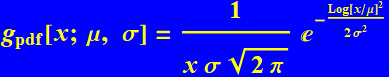 (R.3.6)
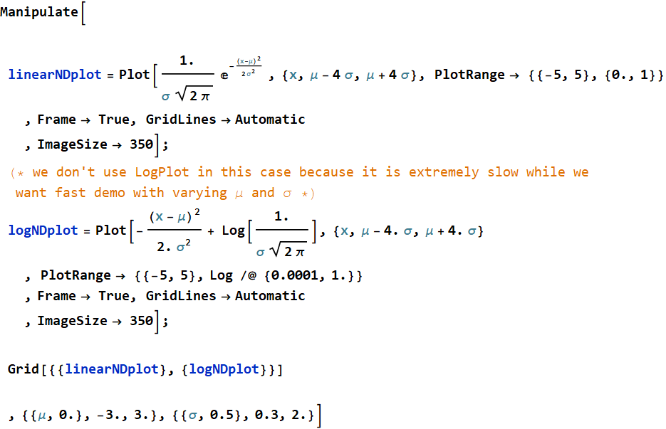
Exercise - Plot normal distribution
Make normal distribution plots on linear scale and log scale with variable input μ and σ. What shape do you observe on log scale. (hint:  ; check on inverted parabola)
Answer
3.3 Calculation of probability
When we have a continuous probability distribution, like this:
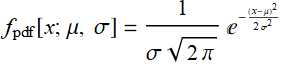 (R.3.5)
It is called pdf: probability density function: it is the probability per unit value of the variable. It is not the probability per se. To compare, consider discrete distribution:
 (R.2.1)
or:
 (R.3.3)
Both ![]() and
and ![]() are probability for event n or m.
are probability for event n or m.
In an exercise above, we are asked how many students get any where from 1-5 tails when flipping coin. We just have to add:
What about continuous distribution like  ?
?
We can’t add, we have to integrate:
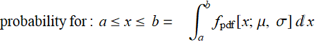 (R .3.6)
For discrete distributions, the sum of all probability values must be 1:
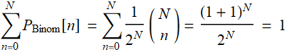 (R.3.7)
and:
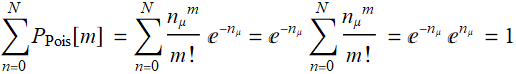 (R.3.8)
For continuous variable, it is the integration over the entire range:
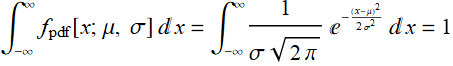 (R.3.9)
Exercise - an illustration of integrating a continuous variable pdf
This exercise is adapted from the supplementary topical lecture on normal distribution.
Here is the app (or you can cut, copy and paste the app onto a new notebook to run outside this notebook while close all active Manipulate cells to make it runs faster).
Run the app to answer the following:
1- What is the probability for a variable (in this case, it is men’s height) to be in 1 standard of deviation (SD) immediately to left or right . Note that if we use unit SD, this calculation is independent of the actual variable: all normal distributions are identical and have the same properties if the mean is shifted to a common fixed value, such as zero, and the unit of length is in SD. In other words, let SD=1.
2- Same as above but this range is 2 SD instead of 1 SD
3- What range, in SD unit, do you get 95% of population or probability (answer in anyway that makes sense to you and there are more than 1 relevant answers)
4- A business website has a well established record that the number of real hits from potential customers/users (not from bots) on a given day is a Poisson distribution with mean ~520. (look up above how a Poisson of mean n can be appoximated as Gaussian with the same mean n, and SD ~ ![]() . Without doing much calculation, just use your result in 3, estimate the range of number of customers/users that you have 95% confidence: which means that there is 95% probability that the number of actual customers/users is inside that range.
. Without doing much calculation, just use your result in 3, estimate the range of number of customers/users that you have 95% confidence: which means that there is 95% probability that the number of actual customers/users is inside that range.
5- Without doing any new calculation but using only the app, estimate the range with your confidence level =75%.
6- One day, the website recorded 590 hits. Usually, there is a well-known ratio of hits vs. orders, but this time, the orders show no statistically significant increase, and you suspect the increase hits are due to bots. What is the probability that 590-and-higher hits are from real potential customers/users? Plot the chance of bot hits as a function of hits above certain level, let that level ranges from 550 to 600.
7- It turns out that it didn’t happen on just one day. Many subsequent days also had high hits. After several days, you find the mean of all hits is now 610. As expected, it is a Poisson distribution also. While you don’t have a way yet to classify real users vs. bots, can you calculate the level of hits at which the chance you have bot hits is equal to the chance you have real customer hits? In other words, what number of hits above which, you think it is higher chance due to bots and below which, it is likely from real customers? (plot the distributions and you will understand the question).
4. Example of applications on financial data
First, you have seen this before in Lesson 2. It is the NASDAQ market index, the symbol is ^IXIC.
The left chart is from 2009 to May 2018. The right chart is a selected period from 8/25/2016 to 12/22/2017 that we choose to study (you can use the date cursor to slide around and zoom in any episode within the date range on the left). Notice the linear behavior on a log scale. It means that the market index grew exponentially (over that episode) vs. time like a compound yield:
![]() (R.4.1)
(R.4.1)
where γ is the yield rate or growth rate.
On log scale, the growth function is: 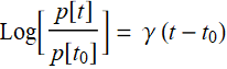 (R.4.2)
which is a linear function.
You will do exercises involving this data. The linear regression fit using Eq. (R.3.2) has been done and the fit graph is given to you as: (it is in the NASDAQ data cell)
![]()
To do this exercise, you need the data in cell below
NASDAQ data (you can open this to take a look, but not necessary, just shift+enter to get data read in)
Exercise - generate a time-series plot
Time-series is the most frequently used plot in finance, economics. Hence, you should start learning how to make it. The function to use is: DateListPlot or DateListLogPlot
Given data ixic, make a time-series plot and name it nasdaqplot
![]()
The above plot is not informative nor stylish. You should try to make one similar the one below, feel free to choose your own color and be creative, but it should show the axes with proper labels
Next, put your plot with the fit plot together like this:
![]()
your answer
Exercise - plot the residual of the fit and its histograms
The deviation between the actual NASDAQ index value and its regression fit is given as . Plot the residuals like the one below. You can choose your own color.
Make 3 histograms: “LogPDF”, “PDF”, and “CDF”. (Go to the app in section R.3.3.3, select lesson 2 to read about CDF). The basic histogram is:
![]()
But you can style your own style and put on proper labels.
your answer
Exercise - fit the histograms with normal distribution
Do this by obtaining the SD of the residual. You will that the mean is ~0 (why?). Then just plot the curves on top each histograms.
your answer
Exercise - buy high - sell low or buy the dip
You have heard “buy the dip” or “sell at the peak” (record, or before the correction) in market strategy. The basic idea is this:
If we truly believe the market is on a steady growth course, one can set a predicted growth rate based on partial history. Then, when the market is below the red growth line, the probablity is that the market would recover eventually, so-called “revert back to the mean” and one can buy. Likewise, when it overshoots, the market would correct and one can sell at high price. Does it really work? it works for those who make money and beat the market, and the same strategy doesn’t work for those who lose.
Why? timing the market is a very difficult task, and if everyone rushes in buying at the dip at the same time, the market responds and it wouldn’t be a dip. If everyone is selling at the peak, the market would dip. In other words, it is not a betting game whose outcome is independent of the betting action, unlike the game betting a man or woman based on one’s height like above, but it is a function of it. This is the theory behind market efficiency. There is a whole field of computation about this, known as stochastic calculus that you will learn later.
For the time being, do a research and write what various schools of investment think and your own thought as well.
5. Normal distribution from central limit theorem
5.1 Discussion
Suppose you have a large number of independent and identically distributed (iid for short) random variables:
array of random variables: ![]() ,
, ![]() ,..
,.. ![]() .
.
and their distribution can be anything, not necessarily normal, as long as they all have a mean ![]() and standard of deviation σ. Then, you take the mean of all of them:
and standard of deviation σ. Then, you take the mean of all of them:
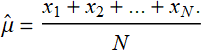
what is the distribution of the mean? The answer from the central limit theorem is:
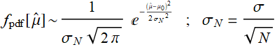
in the limit of large N. In other words, regardless what type of distribution of ![]() , if you take the average of many of them, the more the better, then the average itself would have a Gaussian/ND distribution.
, if you take the average of many of them, the more the better, then the average itself would have a Gaussian/ND distribution.
This central limit theorem is the intuition behind “collecting more data and do average”. Whenever we want to measure something, like the length of an object, or the temperature of a heat or AC outlet, or our weight, we can do it just once. But we might not trust the accuracy and precision of just one measurement (or we hope the 1st weight measurement is way off-scale). We want to do several measurements and take the average (the mean). Why is the average of many is a better measurement than just one single measurement?
The reason is that the standard of deviation of many measurements, like N, is smaller than the standard of deviation of one measurement by  . Do a measurement 10 times, and we are
 ![]() times more confident of the result.
times more confident of the result.
Here is an example. Let’s generate 10 random numbers with uniform distribution between 0 and 1:
![]()
Now we take the mean of that:
![]()
![]()
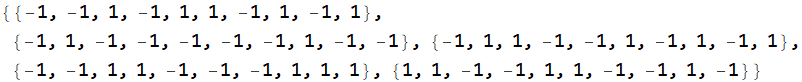
Now, do that say 1000, 2000 ... times and see what the distribution of the mean is. We don’t have to use a do loop for whatever. We can do this: generate 5000 sets of 10 random numbers with one function:

So, xCLT1 above contains 5000 sets, 10 numbers in each set for a total of 50,000 numbers. Here to see it:
![]()
![]()
Here are the first 5 sets:
![]()
| 0.259138 | 0.977064 | 0.699422 | 0.503597 | 0.726496 | 0.563127 | 0.172303 | 0.547116 | 0.467063 | 0.268213 |
| 0.706396 | 0.410744 | 0.650051 | 0.150522 | 0.141692 | 0.250002 | 0.811375 | 0.0748939 | 0.266812 | 0.973922 |
| 0.168161 | 0.155189 | 0.499691 | 0.898753 | 0.692287 | 0.620837 | 0.926317 | 0.891249 | 0.196243 | 0.146431 |
| 0.29102 | 0.588567 | 0.926995 | 0.967232 |