Introduction to probability & Bayes’ rule
ECE generic - segment 1
0. What? Why? (for generic class)
0.1 Problem 1
We have a sensitive and high-precision DVM as shown. We use it to measure the voltage across a resistor. Just the resistor, the whole resistor and nothing but the resistor (no current nor voltage source applied). The voltage is measured at a rate of 100 MS/s. What do you expect to see?
Many students wonder why a square wave signal is “fuzzier” at high frequency (right hand side pict, 0.5 μs/div) than low frequency (left hand side 0.5 ms/div).
0.1.1 Class discussion and demo
0.2 Problem 2
We have a robot that uses a lidar to probe its surrounding. It sends out laser pulses with 1-ns duration. It has a receiver (optical detector) with a responsivity of 0.5 A/W, with a dark current of 1 mA. (0.5-A/W responsivity means that for every watt of optical power incidents on it, it yields 0.5-A current; and 1-mA dark current means that even without any light, i. e. zero optical power, it still yields a steady current of 1 mA).
The robot encounters an object in front of it, but this object is painted black and the backscattered laser pulse power on its receiver is only 0.5 μW. Do you think the robot will be able to tell or will it crash into the obstacle? It can send out many pulses of course. Do you think many pulses will help? and if so, how many pulses will it need to be able to tell if there is an object.
The example below happens all the time:
When a signal is said to be strong or weak, the real question is: strong or weak relative to what? The answer is: relative to the intrinsic noise level of the receiver. Signal-to-noise ratio (SNR) is the most important aspect of a communication link.


Example of clean signal (high SNR) and noisy signal (low SNR) in communications.
0.2.1 Class discussion and demo
0.3 Problem 3
We had a HW as follow: we know the hydrogen atom mass with uncertainty:
![]()
and for the proton: ![]()
We can obtain the electron mass by subtracting ![]() from
from ![]() . What is the electron mass (which is
. What is the electron mass (which is ![]() ) and its uncertainty from this subtraction?
) and its uncertainty from this subtraction?
0.3.1
We can do a similar problem with easier numbers: In the US, men have an average height of 70 inches with a standard of deviation of 4 inches. For women, the figures are 65 inches and 3.5 inches. If we randomly pick, say 1000 men and 1000 women and randomly pair them together to determine the height difference between the man and the woman, what would be the average of this height difference and its standard of deviation?
0.3.2
A problem in a similar vein: Let’s say we have an electrical device (such as an LED or a MOSFET) that has become defective. Instead of drawing a constant current and giving a steady output power, it yields fluctuating power with a Gaussian distribution, with an average (mean) of 10 W and a standard of deviation (SD) of 1 W. We monitor the device voltage and find it too fluctuate with an average of 5 V and a SD of 0.25 V. What is the average current and how much is its fluctuation? in other words, what is the standard of deviation of the device current?
0.4 Problem 4
Consider a robot that is supposed to navigate a disaster area and deliver emergency supplies to victims. It has a locator system (such as GPS and lidar) for navigation. At any moment, it determines its position (using the locator system), calculates which direction and how fast it has to move to reach the victims, and moves until it receives the next update of its location, whence its goes through the cycle of calculation, update, and move again.
Since the locator system has quite a bit of uncertainty, especially in the disaster area with a lot of obstacles, how would you program the robot to use its know capability and information, such as moving with certain speed and direction, with the locator information to find its most optimal way (least erroneous) toward the victims?
Note: This is an example of using Kalman’s filter, and if time permits, we will cover this topic.
0.5 Problem 5

There is a fundamental relationship between risk and reward (yield). High yield investments carry higher volatility and risk than low yield (or no yield) investment. When should you put your money in the bank, or in safe Treasury bills and when you put in the volatile stock market?
In investment, arbitrage is a fundamental process that ensures market efficiency. If a financial instrument is not priced correctly, it is opened to arbitrage. Arbitrage-free pricing is to avoid market inefficiency: two investments with the same yield (payoff) must have the same price (otherwise, arbitrage will occur: buy the cheaper one and sell it for a profit - this happens in every microsecond in the world especially for currency exchange market - so called high-frequency trading).
Likewise, the same with risk: we would never want to invest in something that is high-risk with low pay-off. The payoff must be commensurate with risk. How to calculate this payoff such that it is best in the market. This is a major- if not THE major- problem of portfolio theory in finance.
Note: if time permits, we might cover the calculus of stochastics differential equations (SDE), (also known as stochastic calculus or Itô calculus), and consider Black-Scholes-Merton model of option pricing.
“I can calculate the movements of celestial bodies, but not the madness of men”
-Sir Isaac Newton (on his loss of 20,000 lbs on South Sea stocks)
Key points (takeaways)
All of the above have one property in common: stochasticity: the nature of having more than one possible outcome that is unpredictable, uncertain, or “random”. Stochastics is a concept applied to all such phenomena, events, or settings. (An etymological note: “stochastic” from Greek means guess, or to aim at).
But something being completely non-deterministic doesn’t mean that we can’t know anything or do anything with it. There is a field of math and science to deal with it and we will see that fundamentally, stochasticity can be just as “predictable” and understandable as deterministic physical laws.
The key operational concepts that we need to start are prediction or estimate and confidence.
The objective of applying (learning) the math of stochastics is to be able to estimate or predict some thing with certain level of confidence.
- For example, which of these two statements, a or b in each case below is useful (meaningful):
Case 1
a- According to our design, after pushing the start button, at time t=5 minutes, our drone will be at {x,y,z}={15 meters, 20 meters, 6 meters} or approximately somewhere pretty close there.
b- we can predict with 90% confidence that the position of our robot at time t=5 minutes to be within 0.1 m in every dimension of {x,y,z}={15 meters, 20 meters, 6 meters} (alternatively, we can say: {15 meters, 20 meters, 6 meters} ± 0.1 m)
- Another example, case 2:
a- We expect to have approximately 12,500 customers to visit our store on Black Friday.
b- We predict with 90% confidence that the number of shoppers on Black Friday to be 12,500 ± 600 people.
- Another example, case 3:
a- Our super quantum computer can predict that the market will crash by 20% or more within the next 3 months with a confidence of... 3.1415926535%.
b- We predict that the market can go up if the economy improves and the Fed holds the rate steady; but the market can crash if the World crisis gets worse. On the other, the market can also stay the same if everything stays the same.
Note: b statement is no joke. Market prognosticators say that every single day on TV.
ECE example: telecommunication. (PPT file link)
1. Introduction: probability
1.1 Discussion
Probability is one of the easiest concept to grasp quickly, and yet can be very confusing with more thoughts. Formally, it is a branch of mathematics known as Measure theory. However, we are not concerned about that rigorous math theory here.
Roll a dice, flip a coin, draw a card from a 52-deck. "Chances" are, everytime we do it, we get a different result. We can't say the results with certainty, but we can say the "probability" of getting certain results. Any layperson can say that it's a 50-50 chance to get either head or tail when flipping a coin, 1/6 to get a certain number from1-6 when rolling a dice, and 1/52 to get a specific card.
What is the chance to get a red card? well there are 26 of them out of 42, so it 26/52=50% or 1/2.
What is the chance to get a diamond? 13/52=1/4
What is the chance to get an ace? 4/52=1/13.
What is the chance to get a black ace: 2/52=1/26.
So how is probability is defined in general? If we play a game that has x number of outcomes for N times, and get P times of certain outcome we want. We would say that the probability to get that outcome is ![]() . Is this really probability? Only if we know for sure it is so. Actually, that is NOT the probability, but ONLY an estimate of that probability. We really don't know. We have to try out for infinite number of times and we must assume that everytime we try, the probability is the same. Then, asymptotically, our observation will approach the true value of that probability. See, now we are in a circuitous route of probability definition.
. Is this really probability? Only if we know for sure it is so. Actually, that is NOT the probability, but ONLY an estimate of that probability. We really don't know. We have to try out for infinite number of times and we must assume that everytime we try, the probability is the same. Then, asymptotically, our observation will approach the true value of that probability. See, now we are in a circuitous route of probability definition.
Later on, we’ll see that the assumption that the odd doesn’t change everytime we play the game is called “stationary random process”.
A reason for the possible confusion is that we are mixing up probability as a mathematical concept and probability in the empirical sense. Heart disease is among the #1 killer. Does it mean that we all have equal chance of dying of heart disease? No, some are heart-healthier than others (e. g. not carrying alleles - variants of genes susceptible to heart-disease, lower cholesterol, good living habits,...) and would have a lower chance than the others. Thus, interpreting the rate of death by heart disease from the empirical data of a large population - a statistics of an ensemble, to predict the chance of a single specific individual to have heart disease is meaningless - except when that “individual” is NOT someone real, but only a hypothetical representative of that population.
Probability is a mathematical concept aimed to describe many empirical phenomena. We just have to understand the underlying assumption when using this math. The theory of probability is a part of the mathematics of measure theory.
1.2 Definition of probability of discrete finite variable
In general, we say that the result (or outcome) of any event in the examples above is a random variable. Those random variables in the examples are discrete and finite. Each can only have a certain result that belongs to a set of finite elements.
So for the dice, the set is: {1,2,3,4,5,6}. For the coin, the set is {head, tail}. For the card, its the 52 cards.
But random variable doesn't have to have a finite set of results. It can be infinite as well.
In any case, if X is the set of outcomes: ![]() , then it is assumed that there is a measure called probability mass function for this outcome:
, then it is assumed that there is a measure called probability mass function for this outcome: ![]() where
where ![]() is defined as the probabilityfor the outcome
is defined as the probabilityfor the outcome ![]() . The sum of all probability must be 1:
. The sum of all probability must be 1:  , and
, and ![]() .
.
1.3 Definition of probability of continuous variable
Far more relevant to physical science is random continuous variable. Any physical quantities, voltage, current, power, temperature, pressure, or kinetic variables such as position, velocity, acceleration, and time of some objects or events,... can be random variables. We have considered some examples in the above.
The voltage/current across of any device can fluctuate randomly from the expected controlled value. This is what we call noise. Even the voltage across a resistor fluctuates: thermal noise (Johnson-Nyquist noise).
Suppose we measure the voltage of some device, tally all the measurements and observe this (these graphs are known as histograms).
|
 |
 |
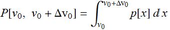
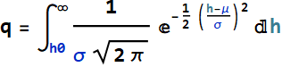
From left to right, we decrease the bin size. If we collect infinite number of samples and arbitrarily decrease the bin size to infinitesimal, we expect to asymptotically reach a continuous curve p[v] as shown in red. This curve is defined as the probability density function which can tell us the probability of measuring a voltage between ![]() and
and ![]() is:
is:
We expect that the probability for a voltage to be between -∞ and ∞ to be 1:
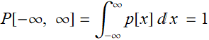
Of course the distribution can be over any range, any combination of intervals and doesn’t have to be [-∞, ∞].
Let’s consider another example. What is the time lapse between two successive lightnings in a thunder storm? here, time lapse t is a continuous real variable. Here it can be anywhere from 0 to ∞. It is positive by definition.
In this case, we define p[t] as probability density function: it is not the probability we talk above. p[t] Δt is the probability for the time lapse between 2 successive lightnings to be between t and t+Δt.
Here, the requirement is p[t] ≥ 0 and 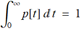 .
.
1.4 Expected value
1.4.1 Examples
Suppose we play the dice with a payoff function as follow:
![]()
| outcome | ||||||
| win/loss | -2 | 2 | -4 | 3 | -5 | 4 |
Suppose the dice is fair. What is the expected win/loss if we play infinite number of games? Intuitively, since each outcome has an equal probability of 1/6, the expected win/loss is:
![]()
This is the expected value of win/loss function per game if we play infinitely and bet the same amount every game. In this case, the player is at a disvantage.
Consider another example. Suppose we have a distribution of children ages at an amusement park as follow:

| age | under 5 | 5 to 10 | above 10 |
| 0.2 | 0.55 | 0.25 | |
| ticket price ($) | 0 | 25 | 40 |
what is the expected earning per kid? Again:
![]()
The expected ticket earning per kid is $23.75.
1.4.2 Formulation
Hence, we can formulate the concept of expected value of a function as follow:
Let ![]() be the probability for each outcome
be the probability for each outcome
Given function of interest: ![]()
The expected value of f is:  or a dot product: P. f
If the distribution is continuous, then:
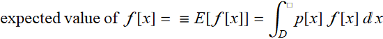 where D is the domain of p[x]
There are two most important expected values:
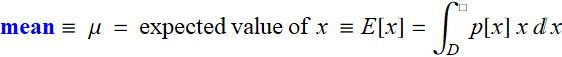
and variance:

Exercise
Consider kids attending an amusement park with this distribution of height:
For one popular ride, there is a height restriction: only kids above 48 inches is allowed for safety reason. Assume every kid who qualifies tries to get on that ride, what is the expected mean height of kids on that ride?
Answer
The PDF of kids on that ride is simply:
![]() and 0 otherwise.
and 0 otherwise.
and 
Thus:
We can rewrite the result:
The mean is:
Just a little albegra to make the result neater:
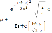
Hence, the mean age of kids on that ride is:
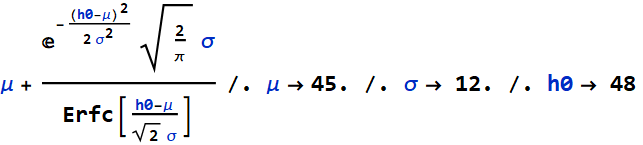
![]()
The mean height is 56.5 inches.
2. Measure theory of probability (optional for ECE 3340)
2.1 Introduction
If we really think about it, when we say we want to know the probability of something, like getting ![]() when rolling a dice
when rolling a dice  , what it means is that we “measure” the chance for that event. Measure theory is the formal name of the branch of mathematics dealing with probability. But we don’t need to know it like a mathematician for our interest, which is engineering applications. This section is to summarize the key concepts, without having to worry about being mathematically rigorous. If you want to skip this section, you can still learn enough about probability for practical applications without being bogged down.
Let’s consider the concept of measure by taking a look in the demo below. Are functions Cos[x], Sin[x] measurements? What do Cos[x], Sin[x] measure here?
2.1.1 example
Clearly, Cos[x], Sin[x] are functions that measure the projection of the rotating radial arm onto x- and y-axis. So, measure is like a function, which is a mapping:
Cos maps the field of complex number ![]() into [-A A] interval of Real number set R.
into [-A A] interval of Real number set R.
2.1.2 Probability is a mapping measure
Thus, we can think of this: probability is also a measure, the measure of chance, which - like a function- is a mapping:
P : event of interest → [0, 1]
But what is the set of events of interest? For a dice, it may appear obvious, the events are:
Ω={![]() ,
,![]() ,
,![]() ,
,![]() ,
,![]() ,
,![]() }
}
where we define the set of all 6 faces as the “sample space”, denoted by Ω. Given the assumption of a fair dice, each face has a chance of ![]()
But is that all? No. The purpose of probability theory is to measure the chances of all events that can be defined beyond those events in the sample space. Why? What do we mean by that? Let’s take a look at this roulette table:
For every spin, there is ONLY ONE - UNIQUE physical outcome: the slot that the ball ends up. But is there only one way to bet? which is where the ball is? No. You can bet:
1- red or black
2- even or odd
3- low: 1-18 or high: 19-36
4- low 3rd: 1-12, mid 3rd: 13-24, high 3rd: 25-36
5- (row or column) set 1: {1,4,...34}, set 2: {2,...35}, set 3: {3,...36}.
6- 0 or 00.
7- finally, the number itself from 1-36 that is not 0 or 00
You see, outcome (which slot the ball is in) can be distinguished from the concept of “events of interest”, which is what we bet.
The same outcome, e. g. the ball in slot 13, can give quite a few different events of interest to the bettors. To bettors who bet on black, it’s a great event, they are happy. For bettors who bet on high: 19-36, they are disappointed. If you bet both black and odd, you will be very happy. There are different types of winners and losers, not just two types: those who bet on 13 and those who don’t.
The purpose of the measure theory of probability is to calculate your odd of winning based on your betting interest, not the unique physical outcome. In other words, you want to know, “I bet on lower 3rd, what is my chance of winning,” (6/19) and not “what is the chance for the ball to be in slot 13.”
The way to do this, in mathematical language, is to define the set of all such events (“the set of all possible betting games”) and calculate the probablity of every element of the set. This set is called a σ-field, (or σ-algebra) denoted by symbol F . Instead of getting into the arcane formal mathematical definition of σ-field F, we will use a more light-hearted and intuitive concept to describe it just like the roulette game; but for simplicity, we will use the dice rather than the roulette.
2.1.3 Example with dice
Note: If the reader skips the discussion with the roulette example, this discussion aims to cover the concept again with the dice with a reasonable number of elements to completely list the σ-field F.
Let’s consider this dice: (known as Chinese dice, as 1 and 4 are red-colored; we make another modification by letting 3 and 6 be blue).
Clearly, when we roll the dice, we get one outcome out of the set of outcomes:
Ω={![]() ,
,![]() ,
,![]() ,
,![]() ,
,![]() ,
,![]() }
}
But that’s not all the possible outcomes that we can use for gambling. As we can see below, certainly we can make many betting games out of it just like roulette.
2.1.4 Betting games with a dice
Here are different ways to set up bet (the more way for a fool to part with his money, the better is for the house). Straight up number bet. Here is the most basic game we can play: you can bet a face out of 6. Win: dice hits your bet.

Odd or even. Win: dice is odd or even
High or low: Win: dice is 4 and above or 3 and below
Win if dice is Red (1, 4), Black (2, 5), or Blue (3, 6)
Take dice face, multiply with its opposit side, bet on the resulting product: 6, 10, or 12 
Or even as simple as this: you win if red, lose otherwise
Or if a prime number (1, 2, 3, 5)....

And so on...
What does the above tell us? When we roll a dice, it is not enough to know the probability of just the unique outcome of each element of set Ω={![]() ,
,![]() ,
,![]() ,
,![]() ,
,![]() ,
,![]() }.
}.
Depending of the game we play, we want to know other events of interest: odd or even, high or low, red, black or blue, etc. and these are beyond the outcomes of just the sample set Ω.
The objective of the theory of probability is to know all possible outcomes which form a set that is built on the basic direct outcomes. For example, in this game:
we don’t care the exact number on the dice face. All we care is whether the result of the dice roll belongs to this set: HIGH={![]() ,
,![]() ,
,![]() }, or LOW= {
}, or LOW= {![]() ,
,![]() ,
,![]() }.
}.
We can refer to HIGH or LOW above as an event of interest, which, along with all other sets of all possible betting gamse constitute the σ-field F.
Clearly, each element of F is a subset of the set of all outcomes Ω={![]() ,
,![]() ,
,![]() ,
,![]() ,
,![]() ,
,![]() }.
}.
Another example: the EVEN set is ={![]() ,
,![]() ,
,![]() } is a subset of Ω. In this game, we don’t care exactly the value of the dice, just whether it is even or odd. The probability of interest here is
} is a subset of Ω. In this game, we don’t care exactly the value of the dice, just whether it is even or odd. The probability of interest here is ![]()
Let’s consider game PRIME. If we bet on it, the outcome of our interest is this set:
PRIME={![]() ,
,![]() ,
,![]() ,
,![]() } which is of course, another subset of Ω. The odd is
} which is of course, another subset of Ω. The odd is ![]() .
.
2.1.5 The σ-field or σ-algebra F of the dice
Now, we can use Mathematica to get all the elements of σ-field F:
![Graphics:PlotLabel /. Options[{RowBox[{RowBox[{Ω, =, RowBox[{{, RowBox[{GraphicsBox[TagBox[RasterBox[RawArray[UnsignedInteger8, <179,177,4>], {{0, 179}, {177, 0}}, {0, 255}, ColorFunction -> RGBColor], BoxForm`ImageTag[System`Convert`CommonDump`ConvertText[Byte, System`Convert`HTMLDump`htmlsave, HTMLEntities -> {HTMLBasic}, AltMathOutput -> PlotLabel, WindowSize -> {2000, Automatic}, MathOutput -> PNG, ConvertClosed -> False, ConvertReverseClosed -> False, ConvertLinkedNotebooks -> False, CharacterEncoding -> Automatic, ConversionStyleEnvironment -> None, ConversionRules -> Automatic, HeadAttributes -> {}, HeadElements -> {}, CSS -> Automatic, ConvertLinkedNotebooks -> False, MathOutput -> GIF, GraphicsOutput -> GIF, Graphics3DOutput -> Automatic, ManipulateOutput -> CDF, ConvertClosed -> True, ConvertReverseClosed -> False, FullDocument -> True, AltMathOutput -> FileName, TableOutput -> {TextForm, Automatic}, AnimationOutput -> Automatic, FilesDirectory -> HTMLFiles, LinksDirectory -> HTMLLinks, HTMLEntities -> {HTML}, AllowBlockMathML -> False, ShowStyles -> True, DataUri -> False, MathMLOptions -> {UseUnicodePlane1Characters -> False, IncludeMarkupAnnotations -> False, Entities -> MathML}], ColorSpace -> System`Convert`CommonDump`ConvertText[RGB, System`Convert`HTMLDump`htmlsave, HTMLEntities -> {HTMLBasic}, AltMathOutput -> PlotLabel, WindowSize -> {2000, Automatic}, MathOutput -> PNG, ConvertClosed -> False, ConvertReverseClosed -> False, ConvertLinkedNotebooks -> False, CharacterEncoding -> Automatic, ConversionStyleEnvironment -> None, ConversionRules -> Automatic, HeadAttributes -> {}, HeadElements -> {}, CSS -> Automatic, ConvertLinkedNotebooks -> False, MathOutput -> GIF, GraphicsOutput -> GIF, Graphics3DOutput -> Automatic, ManipulateOutput -> CDF, ConvertClosed -> True, ConvertReverseClosed -> False, FullDocument -> True, AltMathOutput -> FileName, TableOutput -> {TextForm, Automatic}, AnimationOutput -> Automatic, FilesDirectory -> HTMLFiles, LinksDirectory -> HTMLLinks, HTMLEntities -> {HTML}, AllowBlockMathML -> False, ShowStyles -> True, DataUri -> False, MathMLOptions -> {UseUnicodePlane1Characters -> False, IncludeMarkupAnnotations -> False, Entities -> MathML}], Interleaving -> True], Selectable -> False], DefaultBaseStyle -> System`Convert`CommonDump`ConvertText[ImageGraphics, System`Convert`HTMLDump`htmlsave, HTMLEntities -> {HTMLBasic}, AltMathOutput -> PlotLabel, WindowSize -> {2000, Automatic}, MathOutput -> PNG, ConvertClosed -> False, ConvertReverseClosed -> False, ConvertLinkedNotebooks -> False, CharacterEncoding -> Automatic, ConversionStyleEnvironment -> None, ConversionRules -> Automatic, HeadAttributes -> {}, HeadElements -> {}, CSS -> Automatic, ConvertLinkedNotebooks -> False, MathOutput -> GIF, GraphicsOutput -> GIF, Graphics3DOutput -> Automatic, ManipulateOutput -> CDF, ConvertClosed -> True, ConvertReverseClosed -> False, FullDocument -> True, AltMathOutput -> FileName, TableOutput -> {TextForm, Automatic}, AnimationOutput -> Automatic, FilesDirectory -> HTMLFiles, LinksDirectory -> HTMLLinks, HTMLEntities -> {HTML}, AllowBlockMathML -> False, ShowStyles -> True, DataUri -> False, MathMLOptions -> {UseUnicodePlane1Characters -> False, IncludeMarkupAnnotations -> False, Entities -> MathML}], ImageSize -> {44., Automatic}, ImageSizeRaw -> {177, 179}, PlotRange -> {{0, 177}, {0, 179}}], ,, GraphicsBox[TagBox[RasterBox[RawArray[UnsignedInteger8, <179,180,4>], {{0, 179}, {180, 0}}, {0, 255}, ColorFunction -> RGBColor], BoxForm`ImageTag[System`Convert`CommonDump`ConvertText[Byte, System`Convert`HTMLDump`htmlsave, HTMLEntities -> {HTMLBasic}, AltMathOutput -> PlotLabel, WindowSize -> {2000, Automatic}, MathOutput -> PNG, ConvertClosed -> False, ConvertReverseClosed -> False, ConvertLinkedNotebooks -> False, CharacterEncoding -> Automatic, ConversionStyleEnvironment -> None, ConversionRules -> Automatic, HeadAttributes -> {}, HeadElements -> {}, CSS -> Automatic, ConvertLinkedNotebooks -> False, MathOutput -> GIF, GraphicsOutput -> GIF, Graphics3DOutput -> Automatic, ManipulateOutput -> CDF, ConvertClosed -> True, ConvertReverseClosed -> False, FullDocument -> True, AltMathOutput -> FileName, TableOutput -> {TextForm, Automatic}, AnimationOutput -> Automatic, FilesDirectory -> HTMLFiles, LinksDirectory -> HTMLLinks, HTMLEntities -> {HTML}, AllowBlockMathML -> False, ShowStyles -> True, DataUri -> False, MathMLOptions -> {UseUnicodePlane1Characters -> False, IncludeMarkupAnnotations -> False, Entities -> MathML}], ColorSpace -> System`Convert`CommonDump`ConvertText[RGB, System`Convert`HTMLDump`htmlsave, HTMLEntities -> {HTMLBasic}, AltMathOutput -> PlotLabel, WindowSize -> {2000, Automatic}, MathOutput -> PNG, ConvertClosed -> False, ConvertReverseClosed -> False, ConvertLinkedNotebooks -> False, CharacterEncoding -> Automatic, ConversionStyleEnvironment -> None, ConversionRules -> Automatic, HeadAttributes -> {}, HeadElements -> {}, CSS -> Automatic, ConvertLinkedNotebooks -> False, MathOutput -> GIF, GraphicsOutput -> GIF, Graphics3DOutput -> Automatic, ManipulateOutput -> CDF, ConvertClosed -> True, ConvertReverseClosed -> False, FullDocument -> True, AltMathOutput -> FileName, TableOutput -> {TextForm, Automatic}, AnimationOutput -> Automatic, FilesDirectory -> HTMLFiles, LinksDirectory -> HTMLLinks, HTMLEntities -> {HTML}, AllowBlockMathML -> False, ShowStyles -> True, DataUri -> False, MathMLOptions -> {UseUnicodePlane1Characters -> False, IncludeMarkupAnnotations -> False, Entities -> MathML}], Interleaving -> True], Selectable -> False], DefaultBaseStyle -> System`Convert`CommonDump`ConvertText[ImageGraphics, System`Convert`HTMLDump`htmlsave, HTMLEntities -> {HTMLBasic}, AltMathOutput -> PlotLabel, WindowSize -> {2000, Automatic}, MathOutput -> PNG, ConvertClosed -> False, ConvertReverseClosed -> False, ConvertLinkedNotebooks -> False, CharacterEncoding -> Automatic, ConversionStyleEnvironment -> None, ConversionRules -> Automatic, HeadAttributes -> {}, HeadElements -> {}, CSS -> Automatic, ConvertLinkedNotebooks -> False, MathOutput -> GIF, GraphicsOutput -> GIF, Graphics3DOutput -> Automatic, ManipulateOutput -> CDF, ConvertClosed -> True, ConvertReverseClosed -> False, FullDocument -> True, AltMathOutput -> FileName, TableOutput -> {TextForm, Automatic}, AnimationOutput -> Automatic, FilesDirectory -> HTMLFiles, LinksDirectory -> HTMLLinks, HTMLEntities -> {HTML}, AllowBlockMathML -> False, ShowStyles -> True, DataUri -> False, MathMLOptions -> {UseUnicodePlane1Characters -> False, IncludeMarkupAnnotations -> False, Entities -> MathML}], ImageSize -> {45., Automatic}, ImageSizeRaw -> {180, 179}, PlotRange -> {{0, 180}, {0, 179}}], ,, GraphicsBox[TagBox[RasterBox[RawArray[UnsignedInteger8, <177,180,4>], {{0, 177}, {180, 0}}, {0, 255}, ColorFunction -> RGBColor], BoxForm`ImageTag[System`Convert`CommonDump`ConvertText[Byte, System`Convert`HTMLDump`htmlsave, HTMLEntities -> {HTMLBasic}, AltMathOutput -> PlotLabel, WindowSize -> {2000, Automatic}, MathOutput -> PNG, ConvertClosed -> False, ConvertReverseClosed -> False, ConvertLinkedNotebooks -> False, CharacterEncoding -> Automatic, ConversionStyleEnvironment -> None, ConversionRules -> Automatic, HeadAttributes -> {}, HeadElements -> {}, CSS -> Automatic, ConvertLinkedNotebooks -> False, MathOutput -> GIF, GraphicsOutput -> GIF, Graphics3DOutput -> Automatic, ManipulateOutput -> CDF, ConvertClosed -> True, ConvertReverseClosed -> False, FullDocument -> True, AltMathOutput -> FileName, TableOutput -> {TextForm, Automatic}, AnimationOutput -> Automatic, FilesDirectory -> HTMLFiles, LinksDirectory -> HTMLLinks, HTMLEntities -> {HTML}, AllowBlockMathML -> False, ShowStyles -> True, DataUri -> False, MathMLOptions -> {UseUnicodePlane1Characters -> False, IncludeMarkupAnnotations -> False, Entities -> MathML}], ColorSpace -> System`Convert`CommonDump`ConvertText[RGB, System`Convert`HTMLDump`htmlsave, HTMLEntities -> {HTMLBasic}, AltMathOutput -> PlotLabel, WindowSize -> {2000, Automatic}, MathOutput -> PNG, ConvertClosed -> False, ConvertReverseClosed -> False, ConvertLinkedNotebooks -> False, CharacterEncoding -> Automatic, ConversionStyleEnvironment -> None, ConversionRules -> Automatic, HeadAttributes -> {}, HeadElements -> {}, CSS -> Automatic, ConvertLinkedNotebooks -> False, MathOutput -> GIF, GraphicsOutput -> GIF, Graphics3DOutput -> Automatic, ManipulateOutput -> CDF, ConvertClosed -> True, ConvertReverseClosed -> False, FullDocument -> True, AltMathOutput -> FileName, TableOutput -> {TextForm, Automatic}, AnimationOutput -> Automatic, FilesDirectory -> HTMLFiles, LinksDirectory -> HTMLLinks, HTMLEntities -> {HTML}, AllowBlockMathML -> False, ShowStyles -> True, DataUri -> False, MathMLOptions -> {UseUnicodePlane1Characters -> False, IncludeMarkupAnnotations -> False, Entities -> MathML}], Interleaving -> True], Selectable -> False], DefaultBaseStyle -> System`Convert`CommonDump`ConvertText[ImageGraphics, System`Convert`HTMLDump`htmlsave, HTMLEntities -> {HTMLBasic}, AltMathOutput -> PlotLabel, WindowSize -> {2000, Automatic}, MathOutput -> PNG, ConvertClosed -> False, ConvertReverseClosed -> False, ConvertLinkedNotebooks -> False, CharacterEncoding -> Automatic, ConversionStyleEnvironment -> None, ConversionRules -> Automatic, HeadAttributes -> {}, HeadElements -> {}, CSS -> Automatic, ConvertLinkedNotebooks -> False, MathOutput -> GIF, GraphicsOutput -> GIF, Graphics3DOutput -> Automatic, ManipulateOutput -> CDF, ConvertClosed -> True, ConvertReverseClosed -> False, FullDocument -> True, AltMathOutput -> FileName, TableOutput -> {TextForm, Automatic}, AnimationOutput -> Automatic, FilesDirectory -> HTMLFiles, LinksDirectory -> HTMLLinks, HTMLEntities -> {HTML}, AllowBlockMathML -> False, ShowStyles -> True, DataUri -> False, MathMLOptions -> {UseUnicodePlane1Characters -> False, IncludeMarkupAnnotations -> False, Entities -> MathML}], ImageSize -> {44., Automatic}, ImageSizeRaw -> {180, 177}, PlotRange -> {{0, 180}, {0, 177}}], ,, GraphicsBox[TagBox[RasterBox[RawArray[UnsignedInteger8, <176,178,4>], {{0, 176}, {178, 0}}, {0, 255}, ColorFunction -> RGBColor], BoxForm`ImageTag[System`Convert`CommonDump`ConvertText[Byte, System`Convert`HTMLDump`htmlsave, HTMLEntities -> {HTMLBasic}, AltMathOutput -> PlotLabel, WindowSize -> {2000, Automatic}, MathOutput -> PNG, ConvertClosed -> False, ConvertReverseClosed -> False, ConvertLinkedNotebooks -> False, CharacterEncoding -> Automatic, ConversionStyleEnvironment -> None, ConversionRules -> Automatic, HeadAttributes -> {}, HeadElements -> {}, CSS -> Automatic, ConvertLinkedNotebooks -> False, MathOutput -> GIF, GraphicsOutput -> GIF, Graphics3DOutput -> Automatic, ManipulateOutput -> CDF, ConvertClosed -> True, ConvertReverseClosed -> False, FullDocument -> True, AltMathOutput -> FileName, TableOutput -> {TextForm, Automatic}, AnimationOutput -> Automatic, FilesDirectory -> HTMLFiles, LinksDirectory -> HTMLLinks, HTMLEntities -> {HTML}, AllowBlockMathML -> False, ShowStyles -> True, DataUri -> False, MathMLOptions -> {UseUnicodePlane1Characters -> False, IncludeMarkupAnnotations -> False, Entities -> MathML}], ColorSpace -> System`Convert`CommonDump`ConvertText[RGB, System`Convert`HTMLDump`htmlsave, HTMLEntities -> {HTMLBasic}, AltMathOutput -> PlotLabel, WindowSize -> {2000, Automatic}, MathOutput -> PNG, ConvertClosed -> False, ConvertReverseClosed -> False, ConvertLinkedNotebooks -> False, CharacterEncoding -> Automatic, ConversionStyleEnvironment -> None, ConversionRules -> Automatic, HeadAttributes -> {}, HeadElements -> {}, CSS -> Automatic, ConvertLinkedNotebooks -> False, MathOutput -> GIF, GraphicsOutput -> GIF, Graphics3DOutput -> Automatic, ManipulateOutput -> CDF, ConvertClosed -> True, ConvertReverseClosed -> False, FullDocument -> True, AltMathOutput -> FileName, TableOutput -> {TextForm, Automatic}, AnimationOutput -> Automatic, FilesDirectory -> HTMLFiles, LinksDirectory -> HTMLLinks, HTMLEntities -> {HTML}, AllowBlockMathML -> False, ShowStyles -> True, DataUri -> False, MathMLOptions -> {UseUnicodePlane1Characters -> False, IncludeMarkupAnnotations -> False, Entities -> MathML}], Interleaving -> True], Selectable -> False], DefaultBaseStyle -> System`Convert`CommonDump`ConvertText[ImageGraphics, System`Convert`HTMLDump`htmlsave, HTMLEntities -> {HTMLBasic}, AltMathOutput -> PlotLabel, WindowSize -> {2000, Automatic}, MathOutput -> PNG, ConvertClosed -> False, ConvertReverseClosed -> False, ConvertLinkedNotebooks -> False, CharacterEncoding -> Automatic, ConversionStyleEnvironment -> None, ConversionRules -> Automatic, HeadAttributes -> {}, HeadElements -> {}, CSS -> Automatic, ConvertLinkedNotebooks -> False, MathOutput -> GIF, GraphicsOutput -> GIF, Graphics3DOutput -> Automatic, ManipulateOutput -> CDF, ConvertClosed -> True, ConvertReverseClosed -> False, FullDocument -> True, AltMathOutput -> FileName, TableOutput -> {TextForm, Automatic}, AnimationOutput -> Automatic, FilesDirectory -> HTMLFiles, LinksDirectory -> HTMLLinks, HTMLEntities -> {HTML}, AllowBlockMathML -> False, ShowStyles -> True, DataUri -> False, MathMLOptions -> {UseUnicodePlane1Characters -> False, IncludeMarkupAnnotations -> False, Entities -> MathML}], ImageSize -> {45., Automatic}, ImageSizeRaw -> {178, 176}, PlotRange -> {{0, 178}, {0, 176}}], ,, GraphicsBox[TagBox[RasterBox[RawArray[UnsignedInteger8, <178,176,4>], {{0, 178}, {176, 0}}, {0, 255}, ColorFunction -> RGBColor], BoxForm`ImageTag[System`Convert`CommonDump`ConvertText[Byte, System`Convert`HTMLDump`htmlsave, HTMLEntities -> {HTMLBasic}, AltMathOutput -> PlotLabel, WindowSize -> {2000, Automatic}, MathOutput -> PNG, ConvertClosed -> False, ConvertReverseClosed -> False, ConvertLinkedNotebooks -> False, CharacterEncoding -> Automatic, ConversionStyleEnvironment -> None, ConversionRules -> Automatic, HeadAttributes -> {}, HeadElements -> {}, CSS -> Automatic, ConvertLinkedNotebooks -> False, MathOutput -> GIF, GraphicsOutput -> GIF, Graphics3DOutput -> Automatic, ManipulateOutput -> CDF, ConvertClosed -> True, ConvertReverseClosed -> False, FullDocument -> True, AltMathOutput -> FileName, TableOutput -> {TextForm, Automatic}, AnimationOutput -> Automatic, FilesDirectory -> HTMLFiles, LinksDirectory -> HTMLLinks, HTMLEntities -> {HTML}, AllowBlockMathML -> False, ShowStyles -> True, DataUri -> False, MathMLOptions -> {UseUnicodePlane1Characters -> False, IncludeMarkupAnnotations -> False, Entities -> MathML}], ColorSpace -> System`Convert`CommonDump`ConvertText[RGB, System`Convert`HTMLDump`htmlsave, HTMLEntities -> {HTMLBasic}, AltMathOutput -> PlotLabel, WindowSize -> {2000, Automatic}, MathOutput -> PNG, ConvertClosed -> False, ConvertReverseClosed -> False, ConvertLinkedNotebooks -> False, CharacterEncoding -> Automatic, ConversionStyleEnvironment -> None, ConversionRules -> Automatic, HeadAttributes -> {}, HeadElements -> {}, CSS -> Automatic, ConvertLinkedNotebooks -> False, MathOutput -> GIF, GraphicsOutput -> GIF, Graphics3DOutput -> Automatic, ManipulateOutput -> CDF, ConvertClosed -> True, ConvertReverseClosed -> False, FullDocument -> True, AltMathOutput -> FileName, TableOutput -> {TextForm, Automatic}, AnimationOutput -> Automatic, FilesDirectory -> HTMLFiles, LinksDirectory -> HTMLLinks, HTMLEntities -> {HTML}, AllowBlockMathML -> False, ShowStyles -> True, DataUri -> False, MathMLOptions -> {UseUnicodePlane1Characters -> False, IncludeMarkupAnnotations -> False, Entities -> MathML}], Interleaving -> True], Selectable -> False], DefaultBaseStyle -> System`Convert`CommonDump`ConvertText[ImageGraphics, System`Convert`HTMLDump`htmlsave, HTMLEntities -> {HTMLBasic}, AltMathOutput -> PlotLabel, WindowSize -> {2000, Automatic}, MathOutput -> PNG, ConvertClosed -> False, ConvertReverseClosed -> False, ConvertLinkedNotebooks -> False, CharacterEncoding -> Automatic, ConversionStyleEnvironment -> None, ConversionRules -> Automatic, HeadAttributes -> {}, HeadElements -> {}, CSS -> Automatic, ConvertLinkedNotebooks -> False, MathOutput -> GIF, GraphicsOutput -> GIF, Graphics3DOutput -> Automatic, ManipulateOutput -> CDF, ConvertClosed -> True, ConvertReverseClosed -> False, FullDocument -> True, AltMathOutput -> FileName, TableOutput -> {TextForm, Automatic}, AnimationOutput -> Automatic, FilesDirectory -> HTMLFiles, LinksDirectory -> HTMLLinks, HTMLEntities -> {HTML}, AllowBlockMathML -> False, ShowStyles -> True, DataUri -> False, MathMLOptions -> {UseUnicodePlane1Characters -> False, IncludeMarkupAnnotations -> False, Entities -> MathML}], ImageSize -> {44., Automatic}, ImageSizeRaw -> {176, 178}, PlotRange -> {{0, 176}, {0, 178}}], ,, GraphicsBox[TagBox[RasterBox[RawArray[UnsignedInteger8, <178,176,4>], {{0, 178}, {176, 0}}, {0, 255}, ColorFunction -> RGBColor], BoxForm`ImageTag[System`Convert`CommonDump`ConvertText[Byte, System`Convert`HTMLDump`htmlsave, HTMLEntities -> {HTMLBasic}, AltMathOutput -> PlotLabel, WindowSize -> {2000, Automatic}, MathOutput -> PNG, ConvertClosed -> False, ConvertReverseClosed -> False, ConvertLinkedNotebooks -> False, CharacterEncoding -> Automatic, ConversionStyleEnvironment -> None, ConversionRules -> Automatic, HeadAttributes -> {}, HeadElements -> {}, CSS -> Automatic, ConvertLinkedNotebooks -> False, MathOutput -> GIF, GraphicsOutput -> GIF, Graphics3DOutput -> Automatic, ManipulateOutput -> CDF, ConvertClosed -> True, ConvertReverseClosed -> False, FullDocument -> True, AltMathOutput -> FileName, TableOutput -> {TextForm, Automatic}, AnimationOutput -> Automatic, FilesDirectory -> HTMLFiles, LinksDirectory -> HTMLLinks, HTMLEntities -> {HTML}, AllowBlockMathML -> False, ShowStyles -> True, DataUri -> False, MathMLOptions -> {UseUnicodePlane1Characters -> False, IncludeMarkupAnnotations -> False, Entities -> MathML}], ColorSpace -> System`Convert`CommonDump`ConvertText[RGB, System`Convert`HTMLDump`htmlsave, HTMLEntities -> {HTMLBasic}, AltMathOutput -> PlotLabel, WindowSize -> {2000, Automatic}, MathOutput -> PNG, ConvertClosed -> False, ConvertReverseClosed -> False, ConvertLinkedNotebooks -> False, CharacterEncoding -> Automatic, ConversionStyleEnvironment -> None, ConversionRules -> Automatic, HeadAttributes -> {}, HeadElements -> {}, CSS -> Automatic, ConvertLinkedNotebooks -> False, MathOutput -> GIF, GraphicsOutput -> GIF, Graphics3DOutput -> Automatic, ManipulateOutput -> CDF, ConvertClosed -> True, ConvertReverseClosed -> False, FullDocument -> True, AltMathOutput -> FileName, TableOutput -> {TextForm, Automatic}, AnimationOutput -> Automatic, FilesDirectory -> HTMLFiles, LinksDirectory -> HTMLLinks, HTMLEntities -> {HTML}, AllowBlockMathML -> False, ShowStyles -> True, DataUri -> False, MathMLOptions -> {UseUnicodePlane1Characters -> False, IncludeMarkupAnnotations -> False, Entities -> MathML}], Interleaving -> True], Selectable -> False], DefaultBaseStyle -> System`Convert`CommonDump`ConvertText[ImageGraphics, System`Convert`HTMLDump`htmlsave, HTMLEntities -> {HTMLBasic}, AltMathOutput -> PlotLabel, WindowSize -> {2000, Automatic}, MathOutput -> PNG, ConvertClosed -> False, ConvertReverseClosed -> False, ConvertLinkedNotebooks -> False, CharacterEncoding -> Automatic, ConversionStyleEnvironment -> None, ConversionRules -> Automatic, HeadAttributes -> {}, HeadElements -> {}, CSS -> Automatic, ConvertLinkedNotebooks -> False, MathOutput -> GIF, GraphicsOutput -> GIF, Graphics3DOutput -> Automatic, ManipulateOutput -> CDF, ConvertClosed -> True, ConvertReverseClosed -> False, FullDocument -> True, AltMathOutput -> FileName, TableOutput -> {TextForm, Automatic}, AnimationOutput -> Automatic, FilesDirectory -> HTMLFiles, LinksDirectory -> HTMLLinks, HTMLEntities -> {HTML}, AllowBlockMathML -> False, ShowStyles -> True, DataUri -> False, MathMLOptions -> {UseUnicodePlane1Characters -> False, IncludeMarkupAnnotations -> False, Entities -> MathML}], ImageSize -> {45., Automatic}, ImageSizeRaw -> {176, 178}, PlotRange -> {{0, 176}, {0, 178}}]}], }}]}], ;}], , Fσdice = Subsets[Ω] ;, , Fσdice}]](HTMLFiles/Intro_probability_Bayes_segm1_131.gif)
This is the σ-field of the dice. It contains every possible winning event of any arbitrary game you can invent with the roll of a single dice. The probability theory is about how to calculate the chance for every single case (element) of the σ-field. So, what we may think at the beginning that all we care is to know the chance of each event in sample set: Ω={![]() ,
,![]() ,
,![]() ,
,![]() ,
,![]() ,
,![]() } is simply a subset of the σ-field.
} is simply a subset of the σ-field.
The combination of 3 things: {Ω, F, P} is called a probability measure space.
2.1.6 Measure Theory description of probability
Now, we can formally state the definition of probability. The concept requires 3 items, called a probability measure space (or just probability space).
{Ω, F, P};
and probability is a mapping P: P: F → [0, 1]
Wait, how can we have P=0? the only way an outcome has zero probability is that it contains no outcome. Indeed, this is what we call “null” set: Ø={}; P[Ø]=0
In mathematica, a null set is an empty list:
![]()
![]()
In fact, look in the above, Fσdice does contain the empty set, or the null set.
What is the opposite (complement) to null set? it is the set of ALL possible outcomes, which is Ω, and infact, you can see that Ω is the last element of Fσdice in the example above.
What is the probablity of Ω? clearly, P[Ω]=1, because one of the element of Ω={![]() ,
,![]() ,
,![]() ,
,![]() ,
,![]() ,
,![]() } must occur for a roll of the dice.
} must occur for a roll of the dice.
Now, we have completed the basic formulation of probability.
Let’s summarize key aspect of σ-field F. It is also called σ-algebra, for the following abgebraic properties:
- If an element A ∈ F, then ![]() where
where ![]() is the complement of A
is the complement of A
Example, ![]() is an element of F, then
is an element of F, then
![]()
- If A, B ∈ F, then A∩B and A∪B ∈ F
This is obvious for the case here. Example:
![Graphics:PlotLabel /. Options[{RowBox[{RowBox[{A, =, RowBox[{{, RowBox[{GraphicsBox[TagBox[RasterBox[RawArray[UnsignedInteger8, <179,180,4>], {{0, 179}, {180, 0}}, {0, 255}, ColorFunction -> RGBColor], BoxForm`ImageTag[System`Convert`CommonDump`ConvertText[Byte, System`Convert`HTMLDump`htmlsave, HTMLEntities -> {HTMLBasic}, AltMathOutput -> PlotLabel, WindowSize -> {2000, Automatic}, MathOutput -> PNG, ConvertClosed -> False, ConvertReverseClosed -> False, ConvertLinkedNotebooks -> False, CharacterEncoding -> Automatic, ConversionStyleEnvironment -> None, ConversionRules -> Automatic, HeadAttributes -> {}, HeadElements -> {}, CSS -> Automatic, ConvertLinkedNotebooks -> False, MathOutput -> GIF, GraphicsOutput -> GIF, Graphics3DOutput -> Automatic, ManipulateOutput -> CDF, ConvertClosed -> True, ConvertReverseClosed -> False, FullDocument -> True, AltMathOutput -> FileName, TableOutput -> {TextForm, Automatic}, AnimationOutput -> Automatic, FilesDirectory -> HTMLFiles, LinksDirectory -> HTMLLinks, HTMLEntities -> {HTML}, AllowBlockMathML -> False, ShowStyles -> True, DataUri -> False, MathMLOptions -> {UseUnicodePlane1Characters -> False, IncludeMarkupAnnotations -> False, Entities -> MathML}], ColorSpace -> System`Convert`CommonDump`ConvertText[RGB, System`Convert`HTMLDump`htmlsave, HTMLEntities -> {HTMLBasic}, AltMathOutput -> PlotLabel, WindowSize -> {2000, Automatic}, MathOutput -> PNG, ConvertClosed -> False, ConvertReverseClosed -> False, ConvertLinkedNotebooks -> False, CharacterEncoding -> Automatic, ConversionStyleEnvironment -> None, ConversionRules -> Automatic, HeadAttributes -> {}, HeadElements -> {}, CSS -> Automatic, ConvertLinkedNotebooks -> False, MathOutput -> GIF, GraphicsOutput -> GIF, Graphics3DOutput -> Automatic, ManipulateOutput -> CDF, ConvertClosed -> True, ConvertReverseClosed -> False, FullDocument -> True, AltMathOutput -> FileName, TableOutput -> {TextForm, Automatic}, AnimationOutput -> Automatic, FilesDirectory -> HTMLFiles, LinksDirectory -> HTMLLinks, HTMLEntities -> {HTML}, AllowBlockMathML -> False, ShowStyles -> True, DataUri -> False, MathMLOptions -> {UseUnicodePlane1Characters -> False, IncludeMarkupAnnotations -> False, Entities -> MathML}], Interleaving -> True], Selectable -> False], DefaultBaseStyle -> System`Convert`CommonDump`ConvertText[ImageGraphics, System`Convert`HTMLDump`htmlsave, HTMLEntities -> {HTMLBasic}, AltMathOutput -> PlotLabel, WindowSize -> {2000, Automatic}, MathOutput -> PNG, ConvertClosed -> False, ConvertReverseClosed -> False, ConvertLinkedNotebooks -> False, CharacterEncoding -> Automatic, ConversionStyleEnvironment -> None, ConversionRules -> Automatic, HeadAttributes -> {}, HeadElements -> {}, CSS -> Automatic, ConvertLinkedNotebooks -> False, MathOutput -> GIF, GraphicsOutput -> GIF, Graphics3DOutput -> Automatic, ManipulateOutput -> CDF, ConvertClosed -> True, ConvertReverseClosed -> False, FullDocument -> True, AltMathOutput -> FileName, TableOutput -> {TextForm, Automatic}, AnimationOutput -> Automatic, FilesDirectory -> HTMLFiles, LinksDirectory -> HTMLLinks, HTMLEntities -> {HTML}, AllowBlockMathML -> False, ShowStyles -> True, DataUri -> False, MathMLOptions -> {UseUnicodePlane1Characters -> False, IncludeMarkupAnnotations -> False, Entities -> MathML}], ImageSize -> {45., Automatic}, ImageSizeRaw -> {180, 179}, PlotRange -> {{0, 180}, {0, 179}}], ,, GraphicsBox[TagBox[RasterBox[RawArray[UnsignedInteger8, <176,178,4>], {{0, 176}, {178, 0}}, {0, 255}, ColorFunction -> RGBColor], BoxForm`ImageTag[System`Convert`CommonDump`ConvertText[Byte, System`Convert`HTMLDump`htmlsave, HTMLEntities -> {HTMLBasic}, AltMathOutput -> PlotLabel, WindowSize -> {2000, Automatic}, MathOutput -> PNG, ConvertClosed -> False, ConvertReverseClosed -> False, ConvertLinkedNotebooks -> False, CharacterEncoding -> Automatic, ConversionStyleEnvironment -> None, ConversionRules -> Automatic, HeadAttributes -> {}, HeadElements -> {}, CSS -> Automatic, ConvertLinkedNotebooks -> False, MathOutput -> GIF, GraphicsOutput -> GIF, Graphics3DOutput -> Automatic, ManipulateOutput -> CDF, ConvertClosed -> True, ConvertReverseClosed -> False, FullDocument -> True, AltMathOutput -> FileName, TableOutput -> {TextForm, Automatic}, AnimationOutput -> Automatic, FilesDirectory -> HTMLFiles, LinksDirectory -> HTMLLinks, HTMLEntities -> {HTML}, AllowBlockMathML -> False, ShowStyles -> True, DataUri -> False, MathMLOptions -> {UseUnicodePlane1Characters -> False, IncludeMarkupAnnotations -> False, Entities -> MathML}], ColorSpace -> System`Convert`CommonDump`ConvertText[RGB, System`Convert`HTMLDump`htmlsave, HTMLEntities -> {HTMLBasic}, AltMathOutput -> PlotLabel, WindowSize -> {2000, Automatic}, MathOutput -> PNG, ConvertClosed -> False, ConvertReverseClosed -> False, ConvertLinkedNotebooks -> False, CharacterEncoding -> Automatic, ConversionStyleEnvironment -> None, ConversionRules -> Automatic, HeadAttributes -> {}, HeadElements -> {}, CSS -> Automatic, ConvertLinkedNotebooks -> False, MathOutput -> GIF, GraphicsOutput -> GIF, Graphics3DOutput -> Automatic, ManipulateOutput -> CDF, ConvertClosed -> True, ConvertReverseClosed -> False, FullDocument -> True, AltMathOutput -> FileName, TableOutput -> {TextForm, Automatic}, AnimationOutput -> Automatic, FilesDirectory -> HTMLFiles, LinksDirectory -> HTMLLinks, HTMLEntities -> {HTML}, AllowBlockMathML -> False, ShowStyles -> True, DataUri -> False, MathMLOptions -> {UseUnicodePlane1Characters -> False, IncludeMarkupAnnotations -> False, Entities -> MathML}], Interleaving -> True], Selectable -> False], DefaultBaseStyle -> System`Convert`CommonDump`ConvertText[ImageGraphics, System`Convert`HTMLDump`htmlsave, HTMLEntities -> {HTMLBasic}, AltMathOutput -> PlotLabel, WindowSize -> {2000, Automatic}, MathOutput -> PNG, ConvertClosed -> False, ConvertReverseClosed -> False, ConvertLinkedNotebooks -> False, CharacterEncoding -> Automatic, ConversionStyleEnvironment -> None, ConversionRules -> Automatic, HeadAttributes -> {}, HeadElements -> {}, CSS -> Automatic, ConvertLinkedNotebooks -> False, MathOutput -> GIF, GraphicsOutput -> GIF, Graphics3DOutput -> Automatic, ManipulateOutput -> CDF, ConvertClosed -> True, ConvertReverseClosed -> False, FullDocument -> True, AltMathOutput -> FileName, TableOutput -> {TextForm, Automatic}, AnimationOutput -> Automatic, FilesDirectory -> HTMLFiles, LinksDirectory -> HTMLLinks, HTMLEntities -> {HTML}, AllowBlockMathML -> False, ShowStyles -> True, DataUri -> False, MathMLOptions -> {UseUnicodePlane1Characters -> False, IncludeMarkupAnnotations -> False, Entities -> MathML}], ImageSize -> {45., Automatic}, ImageSizeRaw -> {178, 176}, PlotRange -> {{0, 178}, {0, 176}}], ,, GraphicsBox[TagBox[RasterBox[RawArray[UnsignedInteger8, <178,176,4>], {{0, 178}, {176, 0}}, {0, 255}, ColorFunction -> RGBColor], BoxForm`ImageTag[System`Convert`CommonDump`ConvertText[Byte, System`Convert`HTMLDump`htmlsave, HTMLEntities -> {HTMLBasic}, AltMathOutput -> PlotLabel, WindowSize -> {2000, Automatic}, MathOutput -> PNG, ConvertClosed -> False, ConvertReverseClosed -> False, ConvertLinkedNotebooks -> False, CharacterEncoding -> Automatic, ConversionStyleEnvironment -> None, ConversionRules -> Automatic, HeadAttributes -> {}, HeadElements -> {}, CSS -> Automatic, ConvertLinkedNotebooks -> False, MathOutput -> GIF, GraphicsOutput -> GIF, Graphics3DOutput -> Automatic, ManipulateOutput -> CDF, ConvertClosed -> True, ConvertReverseClosed -> False, FullDocument -> True, AltMathOutput -> FileName, TableOutput -> {TextForm, Automatic}, AnimationOutput -> Automatic, FilesDirectory -> HTMLFiles, LinksDirectory -> HTMLLinks, HTMLEntities -> {HTML}, AllowBlockMathML -> False, ShowStyles -> True, DataUri -> False, MathMLOptions -> {UseUnicodePlane1Characters -> False, IncludeMarkupAnnotations -> False, Entities -> MathML}], ColorSpace -> System`Convert`CommonDump`ConvertText[RGB, System`Convert`HTMLDump`htmlsave, HTMLEntities -> {HTMLBasic}, AltMathOutput -> PlotLabel, WindowSize -> {2000, Automatic}, MathOutput -> PNG, ConvertClosed -> False, ConvertReverseClosed -> False, ConvertLinkedNotebooks -> False, CharacterEncoding -> Automatic, ConversionStyleEnvironment -> None, ConversionRules -> Automatic, HeadAttributes -> {}, HeadElements -> {}, CSS -> Automatic, ConvertLinkedNotebooks -> False, MathOutput -> GIF, GraphicsOutput -> GIF, Graphics3DOutput -> Automatic, ManipulateOutput -> CDF, ConvertClosed -> True, ConvertReverseClosed -> False, FullDocument -> True, AltMathOutput -> FileName, TableOutput -> {TextForm, Automatic}, AnimationOutput -> Automatic, FilesDirectory -> HTMLFiles, LinksDirectory -> HTMLLinks, HTMLEntities -> {HTML}, AllowBlockMathML -> False, ShowStyles -> True, DataUri -> False, MathMLOptions -> {UseUnicodePlane1Characters -> False, IncludeMarkupAnnotations -> False, Entities -> MathML}], Interleaving -> True], Selectable -> False], DefaultBaseStyle -> System`Convert`CommonDump`ConvertText[ImageGraphics, System`Convert`HTMLDump`htmlsave, HTMLEntities -> {HTMLBasic}, AltMathOutput -> PlotLabel, WindowSize -> {2000, Automatic}, MathOutput -> PNG, ConvertClosed -> False, ConvertReverseClosed -> False, ConvertLinkedNotebooks -> False, CharacterEncoding -> Automatic, ConversionStyleEnvironment -> None, ConversionRules -> Automatic, HeadAttributes -> {}, HeadElements -> {}, CSS -> Automatic, ConvertLinkedNotebooks -> False, MathOutput -> GIF, GraphicsOutput -> GIF, Graphics3DOutput -> Automatic, ManipulateOutput -> CDF, ConvertClosed -> True, ConvertReverseClosed -> False, FullDocument -> True, AltMathOutput -> FileName, TableOutput -> {TextForm, Automatic}, AnimationOutput -> Automatic, FilesDirectory -> HTMLFiles, LinksDirectory -> HTMLLinks, HTMLEntities -> {HTML}, AllowBlockMathML -> False, ShowStyles -> True, DataUri -> False, MathMLOptions -> {UseUnicodePlane1Characters -> False, IncludeMarkupAnnotations -> False, Entities -> MathML}], ImageSize -> {44., Automatic}, ImageSizeRaw -> {176, 178}, PlotRange -> {{0, 176}, {0, 178}}], ,, GraphicsBox[TagBox[RasterBox[RawArray[UnsignedInteger8, <178,176,4>], {{0, 178}, {176, 0}}, {0, 255}, ColorFunction -> RGBColor], BoxForm`ImageTag[System`Convert`CommonDump`ConvertText[Byte, System`Convert`HTMLDump`htmlsave, HTMLEntities -> {HTMLBasic}, AltMathOutput -> PlotLabel, WindowSize -> {2000, Automatic}, MathOutput -> PNG, ConvertClosed -> False, ConvertReverseClosed -> False, ConvertLinkedNotebooks -> False, CharacterEncoding -> Automatic, ConversionStyleEnvironment -> None, ConversionRules -> Automatic, HeadAttributes -> {}, HeadElements -> {}, CSS -> Automatic, ConvertLinkedNotebooks -> False, MathOutput -> GIF, GraphicsOutput -> GIF, Graphics3DOutput -> Automatic, ManipulateOutput -> CDF, ConvertClosed -> True, ConvertReverseClosed -> False, FullDocument -> True, AltMathOutput -> FileName, TableOutput -> {TextForm, Automatic}, AnimationOutput -> Automatic, FilesDirectory -> HTMLFiles, LinksDirectory -> HTMLLinks, HTMLEntities -> {HTML}, AllowBlockMathML -> False, ShowStyles -> True, DataUri -> False, MathMLOptions -> {UseUnicodePlane1Characters -> False, IncludeMarkupAnnotations -> False, Entities -> MathML}], ColorSpace -> System`Convert`CommonDump`ConvertText[RGB, System`Convert`HTMLDump`htmlsave, HTMLEntities -> {HTMLBasic}, AltMathOutput -> PlotLabel, WindowSize -> {2000, Automatic}, MathOutput -> PNG, ConvertClosed -> False, ConvertReverseClosed -> False, ConvertLinkedNotebooks -> False, CharacterEncoding -> Automatic, ConversionStyleEnvironment -> None, ConversionRules -> Automatic, HeadAttributes -> {}, HeadElements -> {}, CSS -> Automatic, ConvertLinkedNotebooks -> False, MathOutput -> GIF, GraphicsOutput -> GIF, Graphics3DOutput -> Automatic, ManipulateOutput -> CDF, ConvertClosed -> True, ConvertReverseClosed -> False, FullDocument -> True, AltMathOutput -> FileName, TableOutput -> {TextForm, Automatic}, AnimationOutput -> Automatic, FilesDirectory -> HTMLFiles, LinksDirectory -> HTMLLinks, HTMLEntities -> {HTML}, AllowBlockMathML -> False, ShowStyles -> True, DataUri -> False, MathMLOptions -> {UseUnicodePlane1Characters -> False, IncludeMarkupAnnotations -> False, Entities -> MathML}], Interleaving -> True], Selectable -> False], DefaultBaseStyle -> System`Convert`CommonDump`ConvertText[ImageGraphics, System`Convert`HTMLDump`htmlsave, HTMLEntities -> {HTMLBasic}, AltMathOutput -> PlotLabel, WindowSize -> {2000, Automatic}, MathOutput -> PNG, ConvertClosed -> False, ConvertReverseClosed -> False, ConvertLinkedNotebooks -> False, CharacterEncoding -> Automatic, ConversionStyleEnvironment -> None, ConversionRules -> Automatic, HeadAttributes -> {}, HeadElements -> {}, CSS -> Automatic, ConvertLinkedNotebooks -> False, MathOutput -> GIF, GraphicsOutput -> GIF, Graphics3DOutput -> Automatic, ManipulateOutput -> CDF, ConvertClosed -> True, ConvertReverseClosed -> False, FullDocument -> True, AltMathOutput -> FileName, TableOutput -> {TextForm, Automatic}, AnimationOutput -> Automatic, FilesDirectory -> HTMLFiles, LinksDirectory -> HTMLLinks, HTMLEntities -> {HTML}, AllowBlockMathML -> False, ShowStyles -> True, DataUri -> False, MathMLOptions -> {UseUnicodePlane1Characters -> False, IncludeMarkupAnnotations -> False, Entities -> MathML}], ImageSize -> {45., Automatic}, ImageSizeRaw -> {176, 178}, PlotRange -> {{0, 176}, {0, 178}}]}], }}]}], , ;, , RowBox[{B, =, RowBox[{{, RowBox[{GraphicsBox[TagBox[RasterBox[RawArray[UnsignedInteger8, <179,177,4>], {{0, 179}, {177, 0}}, {0, 255}, ColorFunction -> RGBColor], BoxForm`ImageTag[System`Convert`CommonDump`ConvertText[Byte, System`Convert`HTMLDump`htmlsave, HTMLEntities -> {HTMLBasic}, AltMathOutput -> PlotLabel, WindowSize -> {2000, Automatic}, MathOutput -> PNG, ConvertClosed -> False, ConvertReverseClosed -> False, ConvertLinkedNotebooks -> False, CharacterEncoding -> Automatic, ConversionStyleEnvironment -> None, ConversionRules -> Automatic, HeadAttributes -> {}, HeadElements -> {}, CSS -> Automatic, ConvertLinkedNotebooks -> False, MathOutput -> GIF, GraphicsOutput -> GIF, Graphics3DOutput -> Automatic, ManipulateOutput -> CDF, ConvertClosed -> True, ConvertReverseClosed -> False, FullDocument -> True, AltMathOutput -> FileName, TableOutput -> {TextForm, Automatic}, AnimationOutput -> Automatic, FilesDirectory -> HTMLFiles, LinksDirectory -> HTMLLinks, HTMLEntities -> {HTML}, AllowBlockMathML -> False, ShowStyles -> True, DataUri -> False, MathMLOptions -> {UseUnicodePlane1Characters -> False, IncludeMarkupAnnotations -> False, Entities -> MathML}], ColorSpace -> System`Convert`CommonDump`ConvertText[RGB, System`Convert`HTMLDump`htmlsave, HTMLEntities -> {HTMLBasic}, AltMathOutput -> PlotLabel, WindowSize -> {2000, Automatic}, MathOutput -> PNG, ConvertClosed -> False, ConvertReverseClosed -> False, ConvertLinkedNotebooks -> False, CharacterEncoding -> Automatic, ConversionStyleEnvironment -> None, ConversionRules -> Automatic, HeadAttributes -> {}, HeadElements -> {}, CSS -> Automatic, ConvertLinkedNotebooks -> False, MathOutput -> GIF, GraphicsOutput -> GIF, Graphics3DOutput -> Automatic, ManipulateOutput -> CDF, ConvertClosed -> True, ConvertReverseClosed -> False, FullDocument -> True, AltMathOutput -> FileName, TableOutput -> {TextForm, Automatic}, AnimationOutput -> Automatic, FilesDirectory -> HTMLFiles, LinksDirectory -> HTMLLinks, HTMLEntities -> {HTML}, AllowBlockMathML -> False, ShowStyles -> True, DataUri -> False, MathMLOptions -> {UseUnicodePlane1Characters -> False, IncludeMarkupAnnotations -> False, Entities -> MathML}], Interleaving -> True], Selectable -> False], DefaultBaseStyle -> System`Convert`CommonDump`ConvertText[ImageGraphics, System`Convert`HTMLDump`htmlsave, HTMLEntities -> {HTMLBasic}, AltMathOutput -> PlotLabel, WindowSize -> {2000, Automatic}, MathOutput -> PNG, ConvertClosed -> False, ConvertReverseClosed -> False, ConvertLinkedNotebooks -> False, CharacterEncoding -> Automatic, ConversionStyleEnvironment -> None, ConversionRules -> Automatic, HeadAttributes -> {}, HeadElements -> {}, CSS -> Automatic, ConvertLinkedNotebooks -> False, MathOutput -> GIF, GraphicsOutput -> GIF, Graphics3DOutput -> Automatic, ManipulateOutput -> CDF, ConvertClosed -> True, ConvertReverseClosed -> False, FullDocument -> True, AltMathOutput -> FileName, TableOutput -> {TextForm, Automatic}, AnimationOutput -> Automatic, FilesDirectory -> HTMLFiles, LinksDirectory -> HTMLLinks, HTMLEntities -> {HTML}, AllowBlockMathML -> False, ShowStyles -> True, DataUri -> False, MathMLOptions -> {UseUnicodePlane1Characters -> False, IncludeMarkupAnnotations -> False, Entities -> MathML}], ImageSize -> {44., Automatic}, ImageSizeRaw -> {177, 179}, PlotRange -> {{0, 177}, {0, 179}}], ,, GraphicsBox[TagBox[RasterBox[RawArray[UnsignedInteger8, <176,178,4>], {{0, 176}, {178, 0}}, {0, 255}, ColorFunction -> RGBColor], BoxForm`ImageTag[System`Convert`CommonDump`ConvertText[Byte, System`Convert`HTMLDump`htmlsave, HTMLEntities -> {HTMLBasic}, AltMathOutput -> PlotLabel, WindowSize -> {2000, Automatic}, MathOutput -> PNG, ConvertClosed -> False, ConvertReverseClosed -> False, ConvertLinkedNotebooks -> False, CharacterEncoding -> Automatic, ConversionStyleEnvironment -> None, ConversionRules -> Automatic, HeadAttributes -> {}, HeadElements -> {}, CSS -> Automatic, ConvertLinkedNotebooks -> False, MathOutput -> GIF, GraphicsOutput -> GIF, Graphics3DOutput -> Automatic, ManipulateOutput -> CDF, ConvertClosed -> True, ConvertReverseClosed -> False, FullDocument -> True, AltMathOutput -> FileName, TableOutput -> {TextForm, Automatic}, AnimationOutput -> Automatic, FilesDirectory -> HTMLFiles, LinksDirectory -> HTMLLinks, HTMLEntities -> {HTML}, AllowBlockMathML -> False, ShowStyles -> True, DataUri -> False, MathMLOptions -> {UseUnicodePlane1Characters -> False, IncludeMarkupAnnotations -> False, Entities -> MathML}], ColorSpace -> System`Convert`CommonDump`ConvertText[RGB, System`Convert`HTMLDump`htmlsave, HTMLEntities -> {HTMLBasic}, AltMathOutput -> PlotLabel, WindowSize -> {2000, Automatic}, MathOutput -> PNG, ConvertClosed -> False, ConvertReverseClosed -> False, ConvertLinkedNotebooks -> False, CharacterEncoding -> Automatic, ConversionStyleEnvironment -> None, ConversionRules -> Automatic, HeadAttributes -> {}, HeadElements -> {}, CSS -> Automatic, ConvertLinkedNotebooks -> False, MathOutput -> GIF, GraphicsOutput -> GIF, Graphics3DOutput -> Automatic, ManipulateOutput -> CDF, ConvertClosed -> True, ConvertReverseClosed -> False, FullDocument -> True, AltMathOutput -> FileName, TableOutput -> {TextForm, Automatic}, AnimationOutput -> Automatic, FilesDirectory -> HTMLFiles, LinksDirectory -> HTMLLinks, HTMLEntities -> {HTML}, AllowBlockMathML -> False, ShowStyles -> True, DataUri -> False, MathMLOptions -> {UseUnicodePlane1Characters -> False, IncludeMarkupAnnotations -> False, Entities -> MathML}], Interleaving -> True], Selectable -> False], DefaultBaseStyle -> System`Convert`CommonDump`ConvertText[ImageGraphics, System`Convert`HTMLDump`htmlsave, HTMLEntities -> {HTMLBasic}, AltMathOutput -> PlotLabel, WindowSize -> {2000, Automatic}, MathOutput -> PNG, ConvertClosed -> False, ConvertReverseClosed -> False, ConvertLinkedNotebooks -> False, CharacterEncoding -> Automatic, ConversionStyleEnvironment -> None, ConversionRules -> Automatic, HeadAttributes -> {}, HeadElements -> {}, CSS -> Automatic, ConvertLinkedNotebooks -> False, MathOutput -> GIF, GraphicsOutput -> GIF, Graphics3DOutput -> Automatic, ManipulateOutput -> CDF, ConvertClosed -> True, ConvertReverseClosed -> False, FullDocument -> True, AltMathOutput -> FileName, TableOutput -> {TextForm, Automatic}, AnimationOutput -> Automatic, FilesDirectory -> HTMLFiles, LinksDirectory -> HTMLLinks, HTMLEntities -> {HTML}, AllowBlockMathML -> False, ShowStyles -> True, DataUri -> False, MathMLOptions -> {UseUnicodePlane1Characters -> False, IncludeMarkupAnnotations -> False, Entities -> MathML}], ImageSize -> {45., Automatic}, ImageSizeRaw -> {178, 176}, PlotRange -> {{0, 178}, {0, 176}}], ,, GraphicsBox[TagBox[RasterBox[RawArray[UnsignedInteger8, <178,176,4>], {{0, 178}, {176, 0}}, {0, 255}, ColorFunction -> RGBColor], BoxForm`ImageTag[System`Convert`CommonDump`ConvertText[Byte, System`Convert`HTMLDump`htmlsave, HTMLEntities -> {HTMLBasic}, AltMathOutput -> PlotLabel, WindowSize -> {2000, Automatic}, MathOutput -> PNG, ConvertClosed -> False, ConvertReverseClosed -> False, ConvertLinkedNotebooks -> False, CharacterEncoding -> Automatic, ConversionStyleEnvironment -> None, ConversionRules -> Automatic, HeadAttributes -> {}, HeadElements -> {}, CSS -> Automatic, ConvertLinkedNotebooks -> False, MathOutput -> GIF, GraphicsOutput -> GIF, Graphics3DOutput -> Automatic, ManipulateOutput -> CDF, ConvertClosed -> True, ConvertReverseClosed -> False, FullDocument -> True, AltMathOutput -> FileName, TableOutput -> {TextForm, Automatic}, AnimationOutput -> Automatic, FilesDirectory -> HTMLFiles, LinksDirectory -> HTMLLinks, HTMLEntities -> {HTML}, AllowBlockMathML -> False, ShowStyles -> True, DataUri -> False, MathMLOptions -> {UseUnicodePlane1Characters -> False, IncludeMarkupAnnotations -> False, Entities -> MathML}], ColorSpace -> System`Convert`CommonDump`ConvertText[RGB, System`Convert`HTMLDump`htmlsave, HTMLEntities -> {HTMLBasic}, AltMathOutput -> PlotLabel, WindowSize -> {2000, Automatic}, MathOutput -> PNG, ConvertClosed -> False, ConvertReverseClosed -> False, ConvertLinkedNotebooks -> False, CharacterEncoding -> Automatic, ConversionStyleEnvironment -> None, ConversionRules -> Automatic, HeadAttributes -> {}, HeadElements -> {}, CSS -> Automatic, ConvertLinkedNotebooks -> False, MathOutput -> GIF, GraphicsOutput -> GIF, Graphics3DOutput -> Automatic, ManipulateOutput -> CDF, ConvertClosed -> True, ConvertReverseClosed -> False, FullDocument -> True, AltMathOutput -> FileName, TableOutput -> {TextForm, Automatic}, AnimationOutput -> Automatic, FilesDirectory -> HTMLFiles, LinksDirectory -> HTMLLinks, HTMLEntities -> {HTML}, AllowBlockMathML -> False, ShowStyles -> True, DataUri -> False, MathMLOptions -> {UseUnicodePlane1Characters -> False, IncludeMarkupAnnotations -> False, Entities -> MathML}], Interleaving -> True], Selectable -> False], DefaultBaseStyle -> System`Convert`CommonDump`ConvertText[ImageGraphics, System`Convert`HTMLDump`htmlsave, HTMLEntities -> {HTMLBasic}, AltMathOutput -> PlotLabel, WindowSize -> {2000, Automatic}, MathOutput -> PNG, ConvertClosed -> False, ConvertReverseClosed -> False, ConvertLinkedNotebooks -> False, CharacterEncoding -> Automatic, ConversionStyleEnvironment -> None, ConversionRules -> Automatic, HeadAttributes -> {}, HeadElements -> {}, CSS -> Automatic, ConvertLinkedNotebooks -> False, MathOutput -> GIF, GraphicsOutput -> GIF, Graphics3DOutput -> Automatic, ManipulateOutput -> CDF, ConvertClosed -> True, ConvertReverseClosed -> False, FullDocument -> True, AltMathOutput -> FileName, TableOutput -> {TextForm, Automatic}, AnimationOutput -> Automatic, FilesDirectory -> HTMLFiles, LinksDirectory -> HTMLLinks, HTMLEntities -> {HTML}, AllowBlockMathML -> False, ShowStyles -> True, DataUri -> False, MathMLOptions -> {UseUnicodePlane1Characters -> False, IncludeMarkupAnnotations -> False, Entities -> MathML}], ImageSize -> {44., Automatic}, ImageSizeRaw -> {176, 178}, PlotRange -> {{0, 176}, {0, 178}}]}], }}]}], ;}], , {A∩B, A∪B}}]](HTMLFiles/Intro_probability_Bayes_segm1_151.gif)
![]()
We see that A∩B=![]() and A∪B=
and A∪B=![]() are also element of F.
are also element of F.
Based on the above, empty set Ø and the full set Ω must belong to F, because:
![]() ; and
; and ![]()
An element of F:, for example, ![]() can be thought of as “OR”. Thus, a betting on
can be thought of as “OR”. Thus, a betting on ![]() means that the bet wins if either
means that the bet wins if either ![]() , or
, or ![]() , or
, or ![]() , or
, or ![]() occurs.
occurs.
2.1.7 A further example with programming
Let’s take this opportunity to use Mathematica function MemberQ
![]()
![Graphics:PlotLabel /. Options[{RowBox[{RowBox[{bet, =, RowBox[{{, RowBox[{GraphicsBox[TagBox[RasterBox[RawArray[UnsignedInteger8, <179,177,4>], {{0, 179}, {177, 0}}, {0, 255}, ColorFunction -> RGBColor], BoxForm`ImageTag[System`Convert`CommonDump`ConvertText[Byte, System`Convert`HTMLDump`htmlsave, HTMLEntities -> {HTMLBasic}, AltMathOutput -> PlotLabel, WindowSize -> {2000, Automatic}, MathOutput -> PNG, ConvertClosed -> False, ConvertReverseClosed -> False, ConvertLinkedNotebooks -> False, CharacterEncoding -> Automatic, ConversionStyleEnvironment -> None, ConversionRules -> Automatic, HeadAttributes -> {}, HeadElements -> {}, CSS -> Automatic, ConvertLinkedNotebooks -> False, MathOutput -> GIF, GraphicsOutput -> GIF, Graphics3DOutput -> Automatic, ManipulateOutput -> CDF, ConvertClosed -> True, ConvertReverseClosed -> False, FullDocument -> True, AltMathOutput -> FileName, TableOutput -> {TextForm, Automatic}, AnimationOutput -> Automatic, FilesDirectory -> HTMLFiles, LinksDirectory -> HTMLLinks, HTMLEntities -> {HTML}, AllowBlockMathML -> False, ShowStyles -> True, DataUri -> False, MathMLOptions -> {UseUnicodePlane1Characters -> False, IncludeMarkupAnnotations -> False, Entities -> MathML}], ColorSpace -> System`Convert`CommonDump`ConvertText[RGB, System`Convert`HTMLDump`htmlsave, HTMLEntities -> {HTMLBasic}, AltMathOutput -> PlotLabel, WindowSize -> {2000, Automatic}, MathOutput -> PNG, ConvertClosed -> False, ConvertReverseClosed -> False, ConvertLinkedNotebooks -> False, CharacterEncoding -> Automatic, ConversionStyleEnvironment -> None, ConversionRules -> Automatic, HeadAttributes -> {}, HeadElements -> {}, CSS -> Automatic, ConvertLinkedNotebooks -> False, MathOutput -> GIF, GraphicsOutput -> GIF, Graphics3DOutput -> Automatic, ManipulateOutput -> CDF, ConvertClosed -> True, ConvertReverseClosed -> False, FullDocument -> True, AltMathOutput -> FileName, TableOutput -> {TextForm, Automatic}, AnimationOutput -> Automatic, FilesDirectory -> HTMLFiles, LinksDirectory -> HTMLLinks, HTMLEntities -> {HTML}, AllowBlockMathML -> False, ShowStyles -> True, DataUri -> False, MathMLOptions -> {UseUnicodePlane1Characters -> False, IncludeMarkupAnnotations -> False, Entities -> MathML}], Interleaving -> True], Selectable -> False], DefaultBaseStyle -> System`Convert`CommonDump`ConvertText[ImageGraphics, System`Convert`HTMLDump`htmlsave, HTMLEntities -> {HTMLBasic}, AltMathOutput -> PlotLabel, WindowSize -> {2000, Automatic}, MathOutput -> PNG, ConvertClosed -> False, ConvertReverseClosed -> False, ConvertLinkedNotebooks -> False, CharacterEncoding -> Automatic, ConversionStyleEnvironment -> None, ConversionRules -> Automatic, HeadAttributes -> {}, HeadElements -> {}, CSS -> Automatic, ConvertLinkedNotebooks -> False, MathOutput -> GIF, GraphicsOutput -> GIF, Graphics3DOutput -> Automatic, ManipulateOutput -> CDF, ConvertClosed -> True, ConvertReverseClosed -> False, FullDocument -> True, AltMathOutput -> FileName, TableOutput -> {TextForm, Automatic}, AnimationOutput -> Automatic, FilesDirectory -> HTMLFiles, LinksDirectory -> HTMLLinks, HTMLEntities -> {HTML}, AllowBlockMathML -> False, ShowStyles -> True, DataUri -> False, MathMLOptions -> {UseUnicodePlane1Characters -> False, IncludeMarkupAnnotations -> False, Entities -> MathML}], ImageSize -> {44., Automatic}, ImageSizeRaw -> {177, 179}, PlotRange -> {{0, 177}, {0, 179}}], ,, GraphicsBox[TagBox[RasterBox[RawArray[UnsignedInteger8, <177,180,4>], {{0, 177}, {180, 0}}, {0, 255}, ColorFunction -> RGBColor], BoxForm`ImageTag[System`Convert`CommonDump`ConvertText[Byte, System`Convert`HTMLDump`htmlsave, HTMLEntities -> {HTMLBasic}, AltMathOutput -> PlotLabel, WindowSize -> {2000, Automatic}, MathOutput -> PNG, ConvertClosed -> False, ConvertReverseClosed -> False, ConvertLinkedNotebooks -> False, CharacterEncoding -> Automatic, ConversionStyleEnvironment -> None, ConversionRules -> Automatic, HeadAttributes -> {}, HeadElements -> {}, CSS -> Automatic, ConvertLinkedNotebooks -> False, MathOutput -> GIF, GraphicsOutput -> GIF, Graphics3DOutput -> Automatic, ManipulateOutput -> CDF, ConvertClosed -> True, ConvertReverseClosed -> False, FullDocument -> True, AltMathOutput -> FileName, TableOutput -> {TextForm, Automatic}, AnimationOutput -> Automatic, FilesDirectory -> HTMLFiles, LinksDirectory -> HTMLLinks, HTMLEntities -> {HTML}, AllowBlockMathML -> False, ShowStyles -> True, DataUri -> False, MathMLOptions -> {UseUnicodePlane1Characters -> False, IncludeMarkupAnnotations -> False, Entities -> MathML}], ColorSpace -> System`Convert`CommonDump`ConvertText[RGB, System`Convert`HTMLDump`htmlsave, HTMLEntities -> {HTMLBasic}, AltMathOutput -> PlotLabel, WindowSize -> {2000, Automatic}, MathOutput -> PNG, ConvertClosed -> False, ConvertReverseClosed -> False, ConvertLinkedNotebooks -> False, CharacterEncoding -> Automatic, ConversionStyleEnvironment -> None, ConversionRules -> Automatic, HeadAttributes -> {}, HeadElements -> {}, CSS -> Automatic, ConvertLinkedNotebooks -> False, MathOutput -> GIF, GraphicsOutput -> GIF, Graphics3DOutput -> Automatic, ManipulateOutput -> CDF, ConvertClosed -> True, ConvertReverseClosed -> False, FullDocument -> True, AltMathOutput -> FileName, TableOutput -> {TextForm, Automatic}, AnimationOutput -> Automatic, FilesDirectory -> HTMLFiles, LinksDirectory -> HTMLLinks, HTMLEntities -> {HTML}, AllowBlockMathML -> False, ShowStyles -> True, DataUri -> False, MathMLOptions -> {UseUnicodePlane1Characters -> False, IncludeMarkupAnnotations -> False, Entities -> MathML}], Interleaving -> True], Selectable -> False], DefaultBaseStyle -> System`Convert`CommonDump`ConvertText[ImageGraphics, System`Convert`HTMLDump`htmlsave, HTMLEntities -> {HTMLBasic}, AltMathOutput -> PlotLabel, WindowSize -> {2000, Automatic}, MathOutput -> PNG, ConvertClosed -> False, ConvertReverseClosed -> False, ConvertLinkedNotebooks -> False, CharacterEncoding -> Automatic, ConversionStyleEnvironment -> None, ConversionRules -> Automatic, HeadAttributes -> {}, HeadElements -> {}, CSS -> Automatic, ConvertLinkedNotebooks -> False, MathOutput -> GIF, GraphicsOutput -> GIF, Graphics3DOutput -> Automatic, ManipulateOutput -> CDF, ConvertClosed -> True, ConvertReverseClosed -> False, FullDocument -> True, AltMathOutput -> FileName, TableOutput -> {TextForm, Automatic}, AnimationOutput -> Automatic, FilesDirectory -> HTMLFiles, LinksDirectory -> HTMLLinks, HTMLEntities -> {HTML}, AllowBlockMathML -> False, ShowStyles -> True, DataUri -> False, MathMLOptions -> {UseUnicodePlane1Characters -> False, IncludeMarkupAnnotations -> False, Entities -> MathML}], ImageSize -> {44., Automatic}, ImageSizeRaw -> {180, 177}, PlotRange -> {{0, 180}, {0, 177}}], ,, GraphicsBox[TagBox[RasterBox[RawArray[UnsignedInteger8, <176,178,4>], {{0, 176}, {178, 0}}, {0, 255}, ColorFunction -> RGBColor], BoxForm`ImageTag[System`Convert`CommonDump`ConvertText[Byte, System`Convert`HTMLDump`htmlsave, HTMLEntities -> {HTMLBasic}, AltMathOutput -> PlotLabel, WindowSize -> {2000, Automatic}, MathOutput -> PNG, ConvertClosed -> False, ConvertReverseClosed -> False, ConvertLinkedNotebooks -> False, CharacterEncoding -> Automatic, ConversionStyleEnvironment -> None, ConversionRules -> Automatic, HeadAttributes -> {}, HeadElements -> {}, CSS -> Automatic, ConvertLinkedNotebooks -> False, MathOutput -> GIF, GraphicsOutput -> GIF, Graphics3DOutput -> Automatic, ManipulateOutput -> CDF, ConvertClosed -> True, ConvertReverseClosed -> False, FullDocument -> True, AltMathOutput -> FileName, TableOutput -> {TextForm, Automatic}, AnimationOutput -> Automatic, FilesDirectory -> HTMLFiles, LinksDirectory -> HTMLLinks, HTMLEntities -> {HTML}, AllowBlockMathML -> False, ShowStyles -> True, DataUri -> False, MathMLOptions -> {UseUnicodePlane1Characters -> False, IncludeMarkupAnnotations -> False, Entities -> MathML}], ColorSpace -> System`Convert`CommonDump`ConvertText[RGB, System`Convert`HTMLDump`htmlsave, HTMLEntities -> {HTMLBasic}, AltMathOutput -> PlotLabel, WindowSize -> {2000, Automatic}, MathOutput -> PNG, ConvertClosed -> False, ConvertReverseClosed -> False, ConvertLinkedNotebooks -> False, CharacterEncoding -> Automatic, ConversionStyleEnvironment -> None, ConversionRules -> Automatic, HeadAttributes -> {}, HeadElements -> {}, CSS -> Automatic, ConvertLinkedNotebooks -> False, MathOutput -> GIF, GraphicsOutput -> GIF, Graphics3DOutput -> Automatic, ManipulateOutput -> CDF, ConvertClosed -> True, ConvertReverseClosed -> False, FullDocument -> True, AltMathOutput -> FileName, TableOutput -> {TextForm, Automatic}, AnimationOutput -> Automatic, FilesDirectory -> HTMLFiles, LinksDirectory -> HTMLLinks, HTMLEntities -> {HTML}, AllowBlockMathML -> False, ShowStyles -> True, DataUri -> False, MathMLOptions -> {UseUnicodePlane1Characters -> False, IncludeMarkupAnnotations -> False, Entities -> MathML}], Interleaving -> True], Selectable -> False], DefaultBaseStyle -> System`Convert`CommonDump`ConvertText[ImageGraphics, System`Convert`HTMLDump`htmlsave, HTMLEntities -> {HTMLBasic}, AltMathOutput -> PlotLabel, WindowSize -> {2000, Automatic}, MathOutput -> PNG, ConvertClosed -> False, ConvertReverseClosed -> False, ConvertLinkedNotebooks -> False, CharacterEncoding -> Automatic, ConversionStyleEnvironment -> None, ConversionRules -> Automatic, HeadAttributes -> {}, HeadElements -> {}, CSS -> Automatic, ConvertLinkedNotebooks -> False, MathOutput -> GIF, GraphicsOutput -> GIF, Graphics3DOutput -> Automatic, ManipulateOutput -> CDF, ConvertClosed -> True, ConvertReverseClosed -> False, FullDocument -> True, AltMathOutput -> FileName, TableOutput -> {TextForm, Automatic}, AnimationOutput -> Automatic, FilesDirectory -> HTMLFiles, LinksDirectory -> HTMLLinks, HTMLEntities -> {HTML}, AllowBlockMathML -> False, ShowStyles -> True, DataUri -> False, MathMLOptions -> {UseUnicodePlane1Characters -> False, IncludeMarkupAnnotations -> False, Entities -> MathML}], ImageSize -> {45., Automatic}, ImageSizeRaw -> {178, 176}, PlotRange -> {{0, 178}, {0, 176}}], ,, GraphicsBox[TagBox[RasterBox[RawArray[UnsignedInteger8, <178,176,4>], {{0, 178}, {176, 0}}, {0, 255}, ColorFunction -> RGBColor], BoxForm`ImageTag[System`Convert`CommonDump`ConvertText[Byte, System`Convert`HTMLDump`htmlsave, HTMLEntities -> {HTMLBasic}, AltMathOutput -> PlotLabel, WindowSize -> {2000, Automatic}, MathOutput -> PNG, ConvertClosed -> False, ConvertReverseClosed -> False, ConvertLinkedNotebooks -> False, CharacterEncoding -> Automatic, ConversionStyleEnvironment -> None, ConversionRules -> Automatic, HeadAttributes -> {}, HeadElements -> {}, CSS -> Automatic, ConvertLinkedNotebooks -> False, MathOutput -> GIF, GraphicsOutput -> GIF, Graphics3DOutput -> Automatic, ManipulateOutput -> CDF, ConvertClosed -> True, ConvertReverseClosed -> False, FullDocument -> True, AltMathOutput -> FileName, TableOutput -> {TextForm, Automatic}, AnimationOutput -> Automatic, FilesDirectory -> HTMLFiles, LinksDirectory -> HTMLLinks, HTMLEntities -> {HTML}, AllowBlockMathML -> False, ShowStyles -> True, DataUri -> False, MathMLOptions -> {UseUnicodePlane1Characters -> False, IncludeMarkupAnnotations -> False, Entities -> MathML}], ColorSpace -> System`Convert`CommonDump`ConvertText[RGB, System`Convert`HTMLDump`htmlsave, HTMLEntities -> {HTMLBasic}, AltMathOutput -> PlotLabel, WindowSize -> {2000, Automatic}, MathOutput -> PNG, ConvertClosed -> False, ConvertReverseClosed -> False, ConvertLinkedNotebooks -> False, CharacterEncoding -> Automatic, ConversionStyleEnvironment -> None, ConversionRules -> Automatic, HeadAttributes -> {}, HeadElements -> {}, CSS -> Automatic, ConvertLinkedNotebooks -> False, MathOutput -> GIF, GraphicsOutput -> GIF, Graphics3DOutput -> Automatic, ManipulateOutput -> CDF, ConvertClosed -> True, ConvertReverseClosed -> False, FullDocument -> True, AltMathOutput -> FileName, TableOutput -> {TextForm, Automatic}, AnimationOutput -> Automatic, FilesDirectory -> HTMLFiles, LinksDirectory -> HTMLLinks, HTMLEntities -> {HTML}, AllowBlockMathML -> False, ShowStyles -> True, DataUri -> False, MathMLOptions -> {UseUnicodePlane1Characters -> False, IncludeMarkupAnnotations -> False, Entities -> MathML}], Interleaving -> True], Selectable -> False], DefaultBaseStyle -> System`Convert`CommonDump`ConvertText[ImageGraphics, System`Convert`HTMLDump`htmlsave, HTMLEntities -> {HTMLBasic}, AltMathOutput -> PlotLabel, WindowSize -> {2000, Automatic}, MathOutput -> PNG, ConvertClosed -> False, ConvertReverseClosed -> False, ConvertLinkedNotebooks -> False, CharacterEncoding -> Automatic, ConversionStyleEnvironment -> None, ConversionRules -> Automatic, HeadAttributes -> {}, HeadElements -> {}, CSS -> Automatic, ConvertLinkedNotebooks -> False, MathOutput -> GIF, GraphicsOutput -> GIF, Graphics3DOutput -> Automatic, ManipulateOutput -> CDF, ConvertClosed -> True, ConvertReverseClosed -> False, FullDocument -> True, AltMathOutput -> FileName, TableOutput -> {TextForm, Automatic}, AnimationOutput -> Automatic, FilesDirectory -> HTMLFiles, LinksDirectory -> HTMLLinks, HTMLEntities -> {HTML}, AllowBlockMathML -> False, ShowStyles -> True, DataUri -> False, MathMLOptions -> {UseUnicodePlane1Characters -> False, IncludeMarkupAnnotations -> False, Entities -> MathML}], ImageSize -> {45., Automatic}, ImageSizeRaw -> {176, 178}, PlotRange -> {{0, 176}, {0, 178}}]}], }}]}], ;}], , Grid[{{#, face, did I win?}, {myrollidx = RandomInteger[{1, 6}] , mydice = Ω[[myrollidx]] , MemberQ[bet, mydice]}}, Frame→ All]}]](HTMLFiles/Intro_probability_Bayes_segm1_164.gif)
| # | face | did I win? |
| 2 | False |
code: a simple illustration of a dice game
exercise
We have a game of 3 cups. A single red ball can randomly appear under any cup. What are the σ-field for this sample space?
![]()
exercise
Prove that for a discrete finite sample space with n elements, the number of elements of its σ-field is ![]() .
.
2.2 Venn diagram of events
http://demonstrations.wolfram.com/InteractiveVennDiagrams/
2.2.1 Example with cards
We are done with the dice in 2.1, now let’s play with a 52-card deck.
We draw a card, we get a number and a suit. But if we define our event of interest broader, for example, a red card, then we see that the event can be described in terms of set theory. So if:
A= red card; then B= heart is clearly a subset of A. We write: B⊂A.
If we define C=7, then C doesn't belong to A and neither vice versa. But they do have things in common:
A∩C= {7 and red}={7◊, 7♡} ;
If you use the APP above, this is what you see: 
So we say the A and C intersect, or the intersect of A and C is not a null set.
Two sets may not intersect: for example let D be black aces={A♣, A♠}
Then A∩D=φ: a null set.
Let’s say you need a card that is:
- a figure card (J,Q,K) of any suit
- OR a club with a value divisible by 4.
What is your chance to get that?
If you use the APP, this is what you will see: 
Use this to learn about unions and intersections of many sets.
What is your chance to get a card that is:
1- it is red and divisible by 3 (let’s call this set A)
2- OR, diamond and less than 5 (let’s call this set B)
Also, what is A∩B?
2.3 Probability and measure
2.3.1 Fundamental axioms
In terms of pure mathematics, probability is a measure, it is a value for a given set, obeying the following axioms:
1. p[A] ≥0 ;
2. p[Ω] =1 ; where Ω is the complete set of all events ;
3. If ![]() ,
, ![]() ,
, ![]() , ..
, .. ![]() are mutually exclusive events, then:
are mutually exclusive events, then:
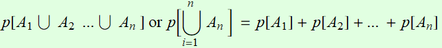
Exercise
Use the card APP. Consider three sets:
A1: ![]() and 10 or below; A2=all
and 10 or below; A2=all ![]() ; and A3= A, K, Q, J of
; and A3= A, K, Q, J of ![]()
- are the sets A1, A2, and A3 mutually exclusive?
- what is P[A1], which is the probability for you to get a ![]() and 10 or below
and 10 or below
- what is P[A2], which is the probability for you to get a ![]()
- what is P[A3], which is the probability for you to get A, K, Q, or J of ![]()
What is the chance for you to get A1, or A2, or A3, which is ![]() ?
?
Is it true that:
![]() ?
?
Exercise
Create an example like the one above with 2 sets B1 and B2 of your choice.
2.3.2 Theorems of belonging and intersection
Theorem: If A⊂B, then p[A]<= p[B].
Since A and B-A are mutually exclusive:
p[A∪ (B-A) ]=p[A]+p[B-A]
p[B]=p[A]+p[B-A]
Since p[B-A]>= 0; then it follows.
Also, since Ø∪Ω=Ω, and Ø∩Ω=Ø, then p[Ω]=p[Ω]+p[Ø]=1 ; it follows: p[Ø]=0.
We define the probability of A∩B as the joint probability of both events A and B; and denote:
p[A∩B] ≡ p[A,B]
Clearly, since A∩B ⊂A and A∩B ⊂B, then p[A,B]<= p[A] and p[B]. These results should be intuitively obvious.
Exercise
Use the card APP.
1- What is the probability to get an A, K, Q, J, or 10 (any suit)
2- What is the probability to get a black card (any face or value)
What is the chance to get a black A, K, Q, J, or 10 based on your results in 1 and 2.
Exercise
You create an example as above.
Theorem: If ![]() ,
, ![]() ,
, ![]() , ..
, .. ![]() are a set of mutually exclusive events, then:
are a set of mutually exclusive events, then:
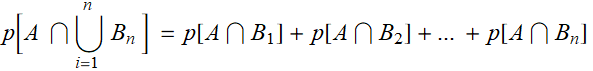
If ![]() ,
, ![]() ,
, ![]() , ..
, .. ![]() are the complete set of all possible events, then
are the complete set of all possible events, then  , and
, and
![]()
Exercise
Use the card APP. Consider three sets:
B1= all even number cards. B2=all odd number cards. B3= all A, K, Q, J
1-Is it true:  ?
?
2- Let A be the set of all diamond cards that are either ace or divisible by 3. what is the probability for A? (this is p[A])
3- What is the chance for each case: A and B1, A and B2, A and B3. (these are: ![]() ,
, ![]() ,
, ![]() )
)
3- Show that
![]()
Exercise
An online store classifies all buyers into 3 categories: 1st-time registered buyer, returning buyer, and guest buyer who doesn’t register and cannot be identified with anyone in the other two categories. They have the following statistics: 1st-time buyer: 25%, returning buyer: 60%. The remaining is for the guest buyer category.
By using data analytics from an independent company, they also know that women buyers make up 70% of all buyers. The rest are men or unknown. Using credit card and name data, they find out further that women make up 80% of first time buyers and 75% of 2nd-time buyers.
1- What is that percentage of women 1st-time buyers relative to ALL buyers.
wft=80% × 25%=
2- What is that percentage of women returning buyers relative to ALL buyers.
3- What is the percentage of men or unknown buyers in the guest buyer category?
4- What is that percentage of men or unknown guest buyers relative to ALL buyers.
Further discussion
See HW. In class discussion.
2.3.3 Theorem of composition
Exercise
What is the probability to get an ace? What is the probability to get an even card (2,4,6,8,10)?
What is the probability to get and ace OR an even card?
Is it true that: P[ace ∪ even card]= P[ace]+ P[even card] ?
Exercise
What is the probability to get a A, K, Q, J? this is P[{A,J,Q,K}]
What is the probability to get a club ![]() that is divisible by 3 (3, 6, 9
that is divisible by 3 (3, 6, 9 ![]() ) this is P[{3
) this is P[{3![]() ,6
,6![]() ,9
,9![]() }]
}]
What is the probability to get {A,J,Q,K} OR {3![]() ,6
,6![]() ,9
,9![]() }
}
Is it true that
![]() ?
?
Exercise
What is the probability to get a A, K, Q, J? this is P[{A,J,Q,K}]
What is the probability to get a heart (any face) ![]() , this is P[{
, this is P[{![]() }]
}]
What is the probability to get {A,J,Q,K} OR {![]() }
}
Is it true that: P[{A,J,Q,K} ∪ {![]() }]= P[{A,J,Q,K}]+ P[{
}]= P[{A,J,Q,K}]+ P[{![]() }] ?
}] ?
Discuss?
In 2.2.1 above, we consider this axiom:
If ![]() ,
, ![]() ,
, ![]() , ..
, .. ![]() are mutually exclusive events, then:
are mutually exclusive events, then:
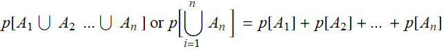
Or for two mutually exclusive events A and B,
p[A∪B] =p[A]+p[B]
and we have done a few exercises on this axiom above.
Now, let A and B be not mutually exclusive. What is p[A∪B] or p[A+B]?
The last Exercise immediately above show that:
![]()
in fact: ![]()
Indeed, intuitively p[A∪B] cannot be as large as p[A] + p[B]. How to calculate it?
http://demonstrations.wolfram.com/InteractiveVennDiagrams/
First, we know that A and B-A are mutually exclusive, and A∪B =A ∪ B-A , hence:
p[A∪B]=p[A]+p[B-A] ≤ p[A] + p[B]
In fact, we can write: A∪B = (A-B) ∪ (A∩B) ∪ (B-A) where the right hand side are all mutually exclusive. Thus:
p[A∪B] = p[A-B] +p[A,B] +p[B-A]
Also: p[A] = p[A-B] +p[A,B] and p[B] = p[B-A] +p[A,B]
Substitute the last two equations into the previous one, we obtain immediately:
p[A∪B] = p[A]+p[B] -p[A,B] : this is known as composition law.
Exercise
Verify that: ![]()
Exercise
Create your own example with cards similar to the Exercise above
Exercise
A click-ad marketing company shows statistics that it reaches 60% of all consumers. On breakdown, it shows that it reaches 35% of consumers via desktop and 50% via mobile platforms. Why is the total of desktop consumers and mobile consumers, 35%+50%=85% is larger than the total online consumers 60%? Estimate the percentage of consumers:
- who use both online and mobile platforms.
- mobile only
- desktop only.
Sketch a diagram to show your explanation.
Exercise
See the same problem as above, but now the marketing company also has statistics on woman and non-woman consumers.
1- It found that 75% of all mobile consumers are women, although women make up only 65% of all the consumers it reaches. How many % its desktop-only consumers are non-women?
2- with the same data as 1 above, the marketing firm further found that 50% desktop users are non-woman. Can you breakdown how many % are mobile-only woman users and how many % are both desktop and mobile woman users?
Exercise
At a thrill ride in an amusement park, for the sake of safety, children are allowed to ride only of they are taller than 45” or weigh more than 60 lbs. Attached is a file of a children group data. Perform the same analysis as in the exercise above and discuss.
Further discussion: Find examples of the composition law
Generally, it can be proven by induction that:
Select a case of your interest, apply composition law and discuss.
E.1 Exercise/lecture - some basic properties of probability density
E.1.1 PDF of a function of a stochastic variable: example
Consider this example. Let the current of a device such as a sensor or some current source be a stochastic variable with Gaussian (Normal) distribution having a mean value μA and standard deviation σA for each measurement interval. We measure it 1000 times, and the result (simulated) is shown below.
This current flows through a resistor R=100 Ω. What is the power of the resistor?
First, we know that:
![]()
If i fluctuates, so must the power. But what is the distribution of power? We can use computer simulation to get the result:
| mean power | SD power |
| 416.712 | 161.878 |
Can we figure out the results of mean and SD without doing simulation? It appears we can guess the mean:
![]()
![]()
which is ~ 400 μW as expected. But what about the SD? Is it:
![]()
![]()
We see that it is not easy to predict the SD with a simple-minded formula. Can we find out why?
The more basic question is: how do we even know what the probability density function (PDF) of power is? Can it be Normal distribution as well? It can’t be, because for a ND, the variable is extended from -∞ to ∞ and power cannot be zero. If so, what distribution is it? It may look like a ND, but not so. Let’s increase the sample population and see:
 |
 |
We see clearly that the power distribution is NOT even a Normal distribution. What is it then?
E.1.2 PDF of a function of a stochastic variable: example discussion
What we want, is to find the probability of power to be in a certain range. To avoid confusion between p[x] for probability density function (PDF) and electrical power, we use symbol u to denote power:
![]() ;
; 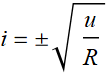
First, consider the positive case  . Then, the probability
 ![]() for u between
for u between ![]() is
is
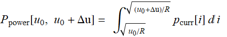
Since  ,
, 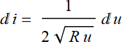 . Thus, we can do a change-of-integration-variable:
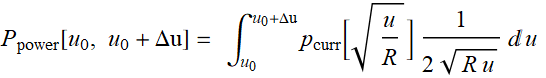
Thus, by definition, the PDF of power is:
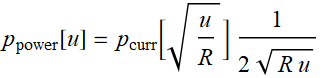
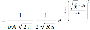
To complete, we have to consider the case  and add both together.
With some trivial algebra, the result for  is (assuming Δu>0)
we can see that adding both cases:
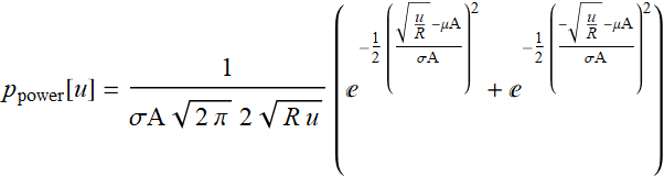
Exercise
The above PDF-> ∞ for u->0. Is it OK?
Answer
It is OK because the integral  is finite. In fact:
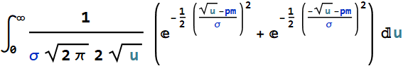
which is 1 as expected.
Exercise
Test the result of ![]() above for the example in E.1.1
above for the example in E.1.1
Answer
E.1.3 PDF of a function of a stochastic variable: general
The above discussion can be generalized on the probability density function (PDF) of any variable that is a function of another stochastic continuous variable. Consider this: let y be a function of stochastic variable x: y=f[x].
Probability for y to be within the yellow stripe ![]() is the sum of all probabilities for x to be within the corresponding intervals
is the sum of all probabilities for x to be within the corresponding intervals ![]() , i from 1 to 4 as illustrated above. For any particular interval, let the local inverse function be:
, i from 1 to 4 as illustrated above. For any particular interval, let the local inverse function be:
x=g[y] ; which can also be written: ![]() (inverse function).
(inverse function).
Then: ![]()
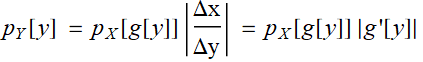
Or: 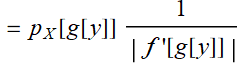
If there are many such intervals, then generally:
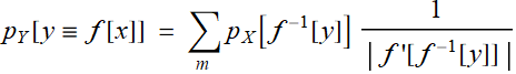
and the summation extends over all points for a multivalue functions. This is exactly what is done in E.1.2
E.1.4 Exercises
Exercise
Let φ be uniformly random between [0, 2π]. What is the distribution of x=a Cos[φ] and y=a Sin[φ]? Do both a numerical simulation and fit with the theoretical curve discussed in E.1.3
Answer
First, we can do numerical simulation:
To derive the PDF:
Check for multi-value cases:
![]()
There are two points to each x interval, hence
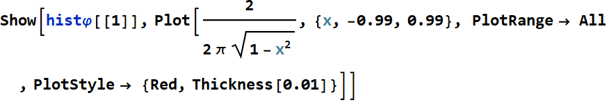
We don’t have to do the same thing for y because sine and cosine over one period is the same, just a phase difference that does not affect the distribution. We can say that x and y have the same distribution.
Exercise
Let the price change of certain commodity, such as gasoline, have Laplace distribution:
δp-> ![]() with α=0.05
with α=0.05
Let the consumption-price elasticity have the form:![]() where q=0.05; r=15 and γ is the price change.
where q=0.05; r=15 and γ is the price change.
![]()
Find the distribution of changes of commodity consumption.
Answer
See HW.
E.1.5 Exercise: PDF involving two or more random variates
Exercise
If we randomly select 5000 men and 5000 women in the US, whose height distributions (from the US CDC data) are ND with the following parameters:
![]()
Find the distribution of the sum and the difference in height using numerical simulation.
 |
 |
Exercise
Consider the voltage and current across a device. Each is a ND with the following properties:
![]()
Do a simulation for 5000 samples and show the distribution of device power. Define equivalent impedance to be voltage/current ratio. Show its distribution. Are these also ND?
Answer
 |
 |
It appears that these are NOT Normal distributions.
Exercise
Consider 2 uniformly distributed variables between 1 and 2. Plot the histograms of their sum and difference,
then, merge both variables into the same set, and plot the histograms of all three.
Answer
Consider another example:
E.1.6 Convolution of PDF
To understand the result of men/women height example in E.1.5 above:
let y=mh+wh
The PDF of y is:
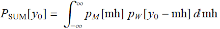
This is a convolution. Recall the Fourier transform theorem:
![]()
We now can apply it. In fact, the Fourier transform of a distribution is called characteristic function, defined as:
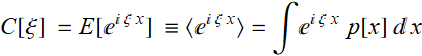
Note that we use both notation E[...] and <...> for expected value, to avoid confusion if there is ambiguity with one of the symbol.
In this case, the characteristic function is:

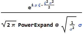

Thus, we take product: ![]()
Define μm+μw≡μS; ![]()

Now, we do inverse Fourier to obtain the convolution:
We see that the distribution is indeed a Normal distribution with mean μS and SD:
![]()
E.1.6.2
For the example with uniform distribution, we use the same approach:

We take the product of the two Fourier transforms:
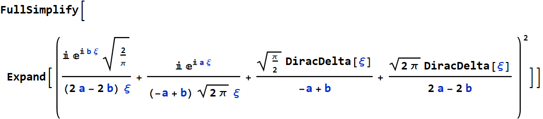
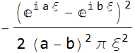
Take the inverse Fourier to obtain the convolution:
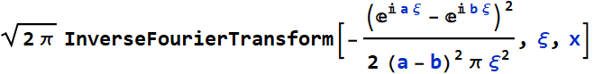

The above function is indeed a triangle like the numerical simulation result:
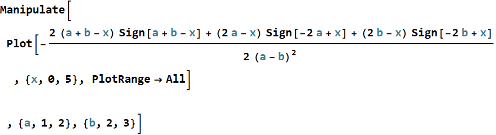
Exercise
Derive the distribution of product and ratio of two Normal distributions.
3. Descriptive statistics - basic concepts
3.1 Introduction
Even without a formal lecture in theory of probability, we all have a basic notion of “average,” which we do all the time. The colloquial expression “on the average...” indicates that even a layperson, non-quantitive person has this notion. Less well known and understood is the concept of variation and distribution. People have ideas that things vary and fluctuate, however, without formal learning, few have concepts of variance or standard of deviation, and even fewer with concepts of skewness and kurtosis.
Here, we’ll go through these basic concepts. It’s important to distinguish two key concepts: estimate and expectation value. These will become clear in the examples below.
3.2 Mean and median
3.2.1 Mean
Instead of the term “average”, we use the term “mean”.
Let’s generate a simulation of height of a population of men according to the US statistics (see the app in other lectures).

![]()
This is how we take the mean of the data above
![]()
![]()
It is NOT equal to μmen=69.2
So, which “mean” is the “mean”?
The value yielded by Mean @ mh5 is “empirical” mean, or “estimated mean”. The mean μmen=69.2 is the expected value what the mean should be as the sample population-> ∞, or “expected mean”.
From 1.4 above, it is:
3.2.2 Median
A clearest and well-known illustration of the difference between mean and median is the case of Lognormal distribution of income, which is the idea behind the cartoon above.
Please go through the app for basic illustration. Select LogNormal distribution to see mean and median.
3.3 Variance, standard of deviation, higher-order moment
HW
3.4 Higher-order moments, skewness and kurtosis
HW
3.5 Histogram, descriptive PDF, CDF
Exercise
The objective of this exercise is to illustrate Laplace transform (PDF, CDF) in a finance example.
Everyday, the stock market can go up or down by certain %. What is the probability p[x] for it to change by x%? The truth is, there is no such known probability. There is no known fundamental law to say what it should be. However, there is the concept of “empirical probability”.
We can obtain this simply by looking at historical data of the % change over a long period, and then make a histogram. Perhaps the shape of the histogram reveals something. This is the “empirical” or “statistical” approach to study a random phenomenon.
3.5.1 Obtain and plot histogram
Import the DJI data given previously (it is on the course webpage). Then find the daily fraction of change and plot a histogram both on linear scale and log scale of PDF (use option “PDF” for linear and {“Log”, “PDF”} for Log). Put in a Manipulate plot with bin width adjustability as well as range adjustability.
Find the mean and variance (not SD).

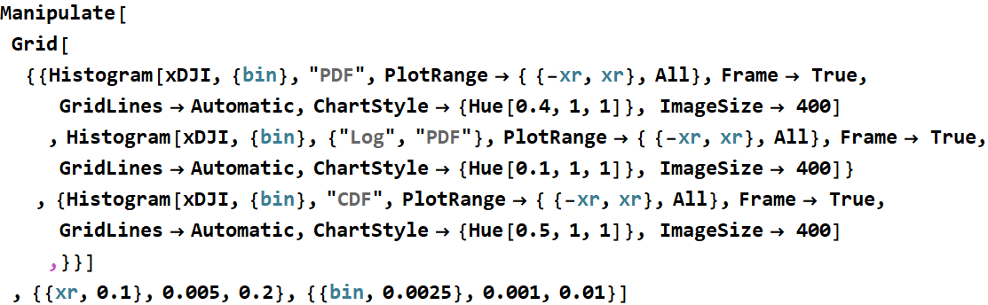
| ^DJI day-to-day change distribution | ||||||
|
3.5.2 Empirical fit
Laplace distribution is defined as:  . Plot the above again with a Laplace distribution on top with asjustable α, set at
  as initial value. Discuss your observation. Note: Think about outlier events that are very rare and may not follow certain expected distribution. Their population is very low and not necessarily significant, but may reflect certain human mass psychology and behavior (“irrational exuberance” vs. mass panic and hysteria).
3.5.3 The sound of the market
You can listen to the market by ListPlay the data you obtain.
![]()
3.5.4 Analyze its power spectral density with the APP
![]()
![]()
3.6 Power spectral density for ordered series
See 3.5.4 above.
3.7 Clusters
See introduction to data analytics.
(cont. to segment 2 - Joint probability, conditional probability & Bayes’ rule - primer)