Introduction to  probability & Bayes’ rule

ECE generic - segment 2

4. Joint probability: a primer

4.1 Examples for concept introduction

4.1.1 Example of finite outcome Ω

Draw a card, suppose we want a black card, the probability is denoted as p[black], the yellow-hi-lited cards below meet the requirement.

Suppose we want a number card that is divisible by 3, we denote the probability as p[div3]. The blue-hi-lited cards below meet the requirement.

Joint probability occurs when we want the probability of not just one feature but multiple features. Thus, if we want a black number card divisible by 3, we call that probability as p[black, div3]: it is the probability to have BOTH requirements, as shown below. They are black cards of 3, 6, 9.

Thus, formally, we can say that the first feature (black card in this example) is subset A in σ-field, and second feature, divisible by 3 is subset B in σ-field, then, the joint probability for both feature is:
                                           p[black, div3]≡p[A,B]=p[A∩B]

Of course we can have more than 2 features. Let’s add a third feature, the number card must be even, then, this is what we have for P[black, div3, even]:  p[black, div3, even]≡p[A,B,C]=P[A∩B∩C], which are just the two black 6 cards as shown below.

4.1.2 Example of continuous variables

We encounter joint probability far more often when dealing with data of real variables. Consider a person’s height, weight, shoulder width, waist size, ... If we have a large group of people, we have a multivariate distribution:
                               p[height, weight, shoulder, waistline,...]
which is a joint-PDF of these variables.

Let’s take a look at a more specific example. Below shows the actual data of a group of people. Each dot is an individual.

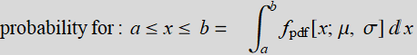
Suppose we want the joint-probability of people with height between 182-186 cm and shoulder width between 40-43 cm. Then, it will be the fraction of people in the rectangle intersection of the two bands as shown.

If we have the PDF: p[h,s], the formal expression is:
                

Of course, the probability integration doesn’t have to be over a rectangle as shown but any domain in the (h,s) space that p[h,s] is integrable.

4.2 Statistical dependence/independence

The most important concepts when having two or more variables or two or more features of interest are “statistical dependence/independence” and “statistically correlation”. These concepts are not relevant if we have only one variable.

Draw a card, we want an ace. That probability is p[ace]. If we want a ◊, that probability is p[◊]. Can we have both? of course, and the probability is p[ace,◊].

But what if I want p[ace, red, ◊]? do we need all three features? no, because ◊ is automatically a part of red. We will say that red is NOT statistically independent of ◊, because if it is a ◊, it MUST be red.

Now, suppose we have continuous variables, such as Form1040 adjusted gross income (AGI) (rounded of to $50 step) and tax. Are they statistically independent? Anyone who pays tax knows the answer: no, death and tax are certainty of life, and the etched-in-stone tax table will say exactly what the tax is for a given AGI. Given a tax, we can inverse lookup what the AGI is. They are statistically dependent on each other.

Let’s measure a car speed with known mass and its kinetic energy. Are speed and KE independent? no, because we know that:    

But far more often, we don’t encounter such clearcut cases of statistical dependence or independence in real life applications. Let’s take a look at the example of human height and shoulder width:

If a person is tall, is it more likely he (the above population is male) has broader shoulder? The data says what common knowledge does: the taller a man is, the more likely will he have a broader shoulder. But given a person’s shoulder width, can we predict exactly what his height is? No, because it has statistical fluctuation. This is a case of statistical correlation, not cut-and-dry dependence/independence discussed above, and it is actually far more common and important in real life applications.

4.3 Statistical correlation or association

Let’s take a look at the figure below for the same example in 4.2:

The height is divided into 7 vertical slices as shown. For each slice, we study shoulder width distribution Note the mean of shoulder width (white red dots) increases vs. height

The white line and white/red point mark the mean of the shoulder width in each slice of height. The gray box marks the [+1 standard of deviation, -1 standard of deviation]  interval. Notice that the mean of shoulder width of each slice of height values increases with increasing height. In other words, the shoulder width is correlated with height

We see that height and shoulder width are NOT completely (or absolutely) independent. Given a height, we can make a guess (inference) what the range of shoulder should be. This is the key concept here: variables that are or are not 100% independent of each other.

In this particular case, we can make a simple linear model: (regression for those who have learned it)
                                       x is the height.                                      

where is height mean, and is the shoulder mean. We don’t know what slope α is but can try to fit visually:

code

There are many similar cases in social science. What is the distribution of income? What is the distribution of height? Is there a corr between income and height? (these are interesting stuffs you can read from time to time in newspapers).

Another example: suppose we collect the following data:
                      p[age, obesity, cholesterol level,frequency of strokes]
Statisticians and epidemiologists love to crank through statistics on the correlation of these things. These research lead to things like:

Other things of popular interest:

There is a whole class of research known as GWAS (Genome Wide Association Studies) if you are curious. Notice that the term “association” is used instead of correlation. The latter is usually used if the relationship is quantitative such as y=a x +b. The former is used for more general relationship that can be either functional or discrete or Boolean (categories).

Example: What genomic features are correlated with income?

The above is just one in the trend of GWAS that includes research such as the below:

Something more amusing:

4.4 Joint-probability axiom and marginal distribution

4.4.1 Joint-probability axiom

In the last example of the above section, we can understand that there is a genetic link to ice cream flavor preference. But let’s consider a study that includes a person’s zip code vs. ice cream flavor, e. g. chocolate or vanilla. Is there any correlation? If we move from one zipcode to another, will we change our ice cream preference? Unlikely!. If so, is there any thing interesting about joint probability p[zipcode, choc/vanil]? Most likely, no. In other words, for any zip code,
                    ;      where is constant  vs. zip code.

If so, should we bother to include zipcode in p[zipcode, choc/vanil]? Obviously, we should not because it is irrelevant. This is why the joint probability distribution of statistically correlated variables is more interesting than either statistical dependence or independence.

The formal axiom on joint probability is that two events will be called statistically independent if and only if
                                                          p[A,B]=p[A].p[B]

Another way to express the concept is that two events are independent when the probablity of occurence of each is the same regardless whether the other occur or not. If A and B are independent, then:
                                                        p[A∩B]=p[A].p[B]

Exercise

1. What is the probability for a card to be red and = 5?  
2. What is the probability of a card to be red and heart?
3. Let’s take 2 cards from a deck of 52; let A= a set of 2 cards that is one red and one black; What is the probability of A?
4. If we take two cards in two different times, each time with a full 52 card deck, what is p[A].
5. Let B be blackjack, excluding double aces. What is p[B]?

Answer

1. What is the probability for a card to be red and = 5?  Probability to be red is 1/2; probability to be 5 is 1/13. So the prob of a card that is red and 5 is:


2. What is the probability of a card to be red and heart? If we use the above principle,
: this is wrong. The reason is that red and heart are NOT independent. Heart is a subset of red. If know a card is a heart, then it must be red. There is no uncertainty. Here we can say that the probability for a card to red if it is known to be a heart is 100%. This is the concept of conditional probability (discussed laler).

3. Let’s take 2 cards from a deck of 52; let A= a set of 2 cards that is one red and one black; What is the probability of A?
                    p[A]= .

4. But now, if we take two cards in two different times, each time with a full 52-card deck, then . We notice that the difference between 1/2 and 26/51 is the fact that in one case, the deck becomes 51 after the first card is drawn.

5. Let B be blackjack, excluding double aces.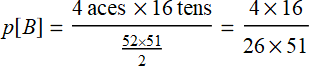

Further discussion:

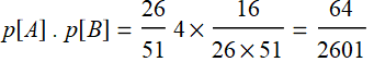
What is the probability for both A and B? (Black jack with one red card and one black card). If A and B were independent:
                             

Is it correct? the probability for a black jack with a red and a black card is:
red aces & black tens + black aces & red tens= 2×2×8
Thus p[A∩B]=

This is NOT the same as p[A] . p[B]

4.4.2 Marginal probability

Consider this example again, If we neglect either one of the two variables, we obtain the PDF of the other variable: this is called marginal PDF.

Each slice of PDF below is also marginal, if we select the height data to be within the indicated range and discard the rest. However, why should we discard the data? A better way to express this is the concept of “conditional probability,” because each slice is conditional that the height be in the domain as indicated.

The height is divided into 7 vertical slices as shown. For each slice, we study shoulder width distribution Note the mean of shoulder width (white red dots) increases vs. height

The white line and white/red point mark the mean of the shoulder width in each slice of height. The gray box marks the [+1 standard of deviation, -1 standard of deviation]  interval. Notice that the mean of shoulder width of each slice of height values increases with increasing height. In other words, the shoulder width is correlated with height

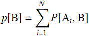
Now, we can discuss marginal propability with formal definition. Let p[A,B] be a joint-distribution, we define the marginal probability as:
                                                 
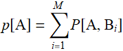
where is the complete set of mutually exclusive events that describe all events of set . Likewise:
                                                 

For continuous real variable, the definition is:
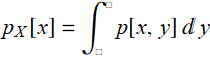                                         and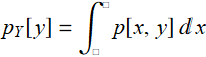        
More generally:  

E.2 Exercise/lecture - multi-variate normal distribution

E.2.1 The importance of multi-variate distribution: an example

Let’s say a clothing manufacturer has big contracts to make school uniforms for two large school systems, say A and B. But it had a terrible manufacturing foul-up: it mixed up two large batches of school uniforms before any decals were sewn-on for identification.

The uniforms are all of different sizes for kids of different ages. And although they may appear similar, the fashion designs are different. School system A uniform has a slightly larger hat, but shorter jacket while school system B has a smaller hat but longer jacket. A casual observer might not know. But not to the fastidious sharp-eye school uniform police who can tell the most minutia fashion details. They would be very upset if the uniforms are wrong.

According to the online-order record and the computerized production system statistics, this is the distribution of hat size and jacket length (relative to the means).

Is it hopeless for the company to salvage the batches by finding a way to discriminate and separate A and B uniforms? They couldn’t afford to randomly send these to the school systems and know they would upset the schools, the parents, and lose their customers once they find out.

It turns out the situation might not be that hopeless.  The good news is, the hat and jacket were packaged together. The mix-up happened after the packaging.  As the company checked the production run, they obtain the joint distribution statistics of hat-and-jacket as shown below:

As one can see, we can draw a line - a discriminant boundary to separate (classify) the two clusters and not a single mix-up if both variables are taken together. What we see here is the effect of “multi-dimensionality” space scaling. The space volumn of a cube of side d grows geometrically ) as a function of number of variables n. If everyone moves on one line, collision will happen. But if we move x and y, we can avoid each other. If we can move x, y, z we can avoid collision even more which is why airplanes don’t collide mid-air as easily as cars. And cars at an intersection with overpasses don’t have accidents as easily as at a path-crossing intersection. (In the above, there is one dimension that is implicit: time - which is why time-multiplexing red/green traffic lights can help avoid data collision).

Airplanes may look dense on 2D, but in reality, they are very very far apart in {x, y, z, t}.

Data in high-dimensional space tend to be rarified and that is the reason why we can classify them into distinct clusters. Clearly, how well we can classify and separate them depends on the distribution.

A very common and straight-forward type of distribution to classify is normal distribution. The game we play in Section 3 in Segment 1 is 1D classification, which requires just one point (although we draw a vertical line, the vertical axis doesn’t mean anything). Here, we will see examples of 2D where the discriminant boundary is truly a 2D line, and 3D with a 3D surface. With generalization to any dimension, the discrimant is an -dimension surface.

E.x  Side note: data input and handling review

While doing exercise 5.2 you may wonder, “is there a quicker and easier way to get parameters and fit a distribution in 5.2”? The answer is yes. If we know the type of distribution, we can use formulas to obtain estimates of parameters which can be used to describe the distribution.

How complex this calculation is depends on the type of distribution. As you might guess, a common type of distribution - and also an easy one to handle - is multivariate normal distribution: it is an extension of the one-D version into higher dimension. You have seen one in 5.3. Since it is a useful distribution, we have this section just for it.

We will use the example of height and shoulder width again. You may wonder why we don’t use an obvious thing like height and weight? The reason is that the distribution of human weight is not Gaussian but lognormal. It is messier mathematically to convolute a Gaussian with lognormal. It is generally true that convolution between any two different distributions is a mess. Of course, numerically, we can program the computer to do anything, but for the learning purpose, the math of Gaussian distribution is the easiest to handle. Both height and should width are length and length of human body tends to have Gaussian distribution.

Here is the data that you should execute to do calculation in subsequent sections.

Data on human body measurements (open up to see details if needed)

In the data cell above, there are two arrays: menbodstat and womenbodstat. Their lengths and dimensions are:

which means there are 247 observations for men, 260 observations for women, each observation has 9 variables. They are:
{age, gender (1=men, 0-woman), height, weight, shouderwidth, pelvic, shouldergirth, chestgirth, waistgirth}

After you read in the data, we are ready to move onto the next.

E .2.1  Covariance matrix and normal distribution fit - Exercise

Exercise - set up data pair height and shoulder width

1- Select height and shoulder width data for men and women (separately) and combine the two variables into a pair. You can name the new data menHS and womenHS. You can do this with Table or Transpose. The first is a bit more intuitive for beginning programmers.

The Transpose method: (you have to use only one, but try to gain an understanding how it works).

Once the data is read-in once,  Transpose method is faster.

2- Make a 3D histogram for each gender, name the histograms menhist3D and womenhist3D, use option “PDF”

your answer

Exercise - obtain the mean and covariance (don’t worry) and plot the fit distribution

If you feel “omg, I forgot what covariance is,” don’t worry, just do it now to get familiar with it and you will learn its details later.

1- Obtain the mean of each gender distribution

2- Instead of variance ( ) for one-dim variable, we obtain the covariance matrix for any data with 2-and-higher D.

men covariance	women covariance

What is the covariance matrix? don’t worry about it for now, just think of it as a complicated form of variance, which is the square of the standard of deviation.

your answer

Exercise - Plot bivariate normal distribution with mean and covariance estimates obtained

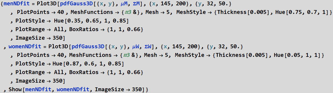
Use this formula and use Plot3D to plot them. μ is the mean and Σ is the covariance matrix you obtain above. Plot 3D distribution for men, for women, and show or plot both together, name the plot: menNDfit, womenNDfit, and menwoND. Plot all on the same range:
{x,145,200},{y,32,50.} so that we can compare. You can choose your own styling.

your answer

Exercise - show the histogram3D you obtain with its Gaussian fit. One for each gender

Observe how the normal distrinbution fit is oriented in a way to cover the histogram as expected with correct aspect of the ellipse and the tilt.

your answer

Exercise - generate simulation with more data points, e. g. 10000

The data above may appear rough fit with its normal distribution. The reason is data insufficiency. If we need 1000 data points to have a smooth fit in 1 D, we would need 1,000,000 data points in 2D. That will take a lot of CPU time. We can do with 10000 points. Use the code developed in 5.2 above, generate 10,000 data points or more and show its histogram with its normal distribution estimate.

your answer

End exercise on binormal distribution of human height and shoulder width

E .2.2  A geometric description of 2D normal distribution

E .2.2.1 General discussion

This section aims to help those who might feel a little uneasy whenever encounter things like “higher dimension” and “matrix”. It is generally true that most can easily grab the concept of single-variable Gaussian or normal distribution (ND) with the familiar bell-shape curve. Yet, the moment “covariant matrix” or ellipsoid are mentioned, things may suddenly appear mysterious.

Below is a simple and succinct approach that uses geometry to describe 2D (bivariate) ND that may help to overcome this sense of unfamiliarity.

code

The key word is variance (or covariance) ellipsoid, which is the essence of a normal distribution and is shown in the plots of the bottom row. The 2D description is generalizable to multi-dimension: in normal distribution, it will be an nth-order ellipsoid surface.

Similarly to one-dimension ND, σ is the distance from the mean where the PDF decreases to or  . It is where: 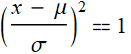                        so that:  

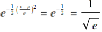
In 2D and higher, the locust of all points that allow an equivalent condition:
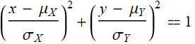              so that:  
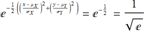
form an ellipse. The variance ellipsoid is the surface where the same condition occurs. Recall this: in an x-y plane, a circle is defined by: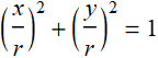            

An ellipsoid is defined by: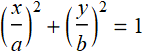                      

To help connecting what we learn in geometry to this case, instead of using notation , , we will use notation {a, b} for major-axis-half-length a and minor-axis-half-length b often.

A circle is an ellipse with a=b=r, the radius. However, there is one thing that the ellipsoid can do that the circle cannot: it can rotate and becomes different, while the circle remains the same if rotated. This simple aspect is actually very important for ND variance ellipsoid: it is related to the correlation of variables which is what you will study in the next section.

E .2.2.2 Explore the app and learn the basic of bivariate normal distribution

The app is not imbedded here since it runs better externally to this lecture. Below is only the icon. Open your app folder to run the stand-alone app (it should be in your app folder).

This is not an app, only the icon of an app. Look in your folder for this app
you will need to run this app to do exercises in E .2.4 and others.

E .2.3 Supplementary math about covariance and the app above

You don’t have to read or study this. This is only for the sake of completeness in explaining the various formula displayed in the app.

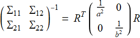
From the App above, you see that the PDF of a bivariate normal distribution can always be transformed with a rotation transformation such that:
        (E .2.3.1a)
                                                                                (E .2.3.1b)
                                                                                            (E .2.3.1c)
                                                            
In other words:
                                                                            (E .2.3.2a)
and 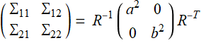                                                                   (E .2.3.2b)
where: 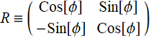                                                                             (E .2.3.2c)
Explicitly:
                                      (E .2.3.3)            

In essence, when you do this rotation in the app:

you can think of having a new system of coordinates:
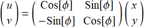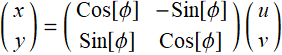        ;                (E .2.3.4)

We will use this result later:
                                      (E .2.3.5)

For simplicity, we have implicitly performed a translation such that and vanish and we can dispense them from all formulas where they are not explicitly needed.

Note that because transformation matrix 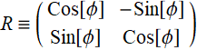  is a unitary matrix:
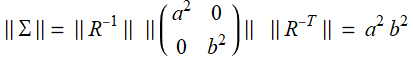                                                  (E .2.3.6)

Thanks to Eq. (E .2.3.1c), we can perform any integration dx dy in the {u, v} space instead:
            dxdy =Jacobian[{x,y};{u,v}] dudv =dudv                                      (E .2.3.7)

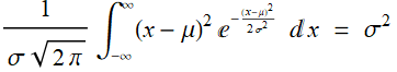
For one-dimensional or one-variable distribution, we define the -moment as
                                  
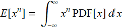
(E stands for expectation - don’t worry for now, it is just a notation convention we follow)
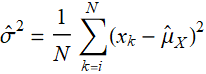
for which, the second moment is defined as the variance:
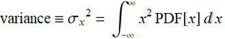                                                                     (E .2.3.8)
With more than one variable, say , ,... , clearly variances of each are not enough to describe the all the quadratic moments that include cross-terms: , k≠j

Thus, besides
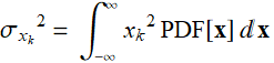                           where              (E .2.3.9)
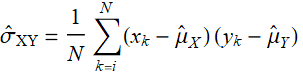
we need the covariance term:
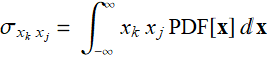                                j≠k                                    (E .2.3.10)
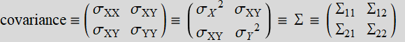
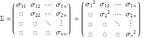
Hence, all variances and covariances form a covariance matrix:
                                 (E .2.3.11a)
More formally in tensor notation, this is also how it is expressed:
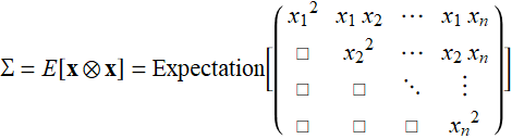                                    (E .2.3.11b)

which, for a bivariate distribution, becomes
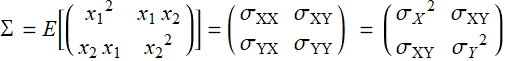                             (E .2.3.12)
We can write for because they are obviously the same for scalar x, y.    

For descriptive statistics, if we have data
then the estimate of the covariance matrix based on (E .2.3.10) is:
                 
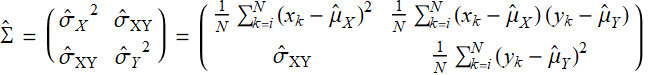
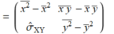                                                                                   (E .2.3.13)
Notice here that we have to put the mean , back into the expression because these are raw data and we have to use different symbols for x and y if we were to make a translation transformation to have new variable x’ y’ for example.

It is well-known that:
                                                           (E .2.3.14)
which is why the estimate for variance is:
                                                                                      (E .2.3.15)

However, if we define the estimate:
                                                                   (E .2.3.16)
How do we integrate:
                   ?                  (E .2.3.17)                               

It is straightforward to integrate in {u,v} space instead:
        
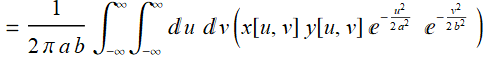                                                    (E .2.3.18)
Making use of Eq. (E .2.3.5) for x y
             

                                                                                       (E .2.3.19)
which is      per Eq. (E .2.3.3).

Hence, this proves (E .2.3.13) is the Bayesian estimate for the covariance matrix.

E .2.4 Exercise of 2D normal distribution

Exercise on shoulder girth and chest girth

Use the data given in E .2.0. Create a data set based on pair {shoulder girth, chest girth}, which are variable 7 and 8. Do one set for men and one set for women. Obtain the covariance matrix for each, which is:
                          
The regression slope between x and y is: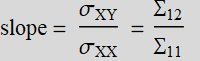         

Then enter the values into the app above () to obtain the ellipsoid representation (copy and paste output of the app into your answer.  Show both the ellipsoid for men and women data on the same graph by using show and select plotrange to be all.

You can read the code below. However, you may not copy and paste. You should write your own code or even type the code below line-by-line, but NO COPY and PASTE: NO Control+x, Control+v

If you show both ellipsoid, this is what you will see (but you must obtain it yourself, this is shown so that you know you are correct).

your answer

Exercise on shoulder girth and chest girth - bivariate normal fit

Plot the bivariate normal distribution fit for each population based on the parameters (mean and covariance) you obtain above. Then put the two normal distributions in the same graphics. You should select different colors for the genders. Better yet, it preferrable that you write your own Plot3D code to plot each or both together. You should obtain something that looks similar to the below. Do you think the distinction between them is large enough to do classification? and what you think how it is compared with just using height alone like what we did in the game?

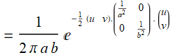
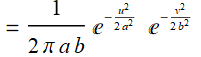
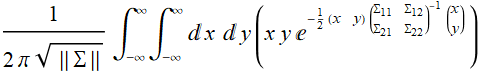
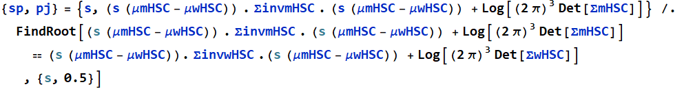
The formula to use with Plot3D is:
                                      
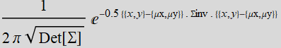
where Σ is the covariance matrix and Σinv is its inverse. Det[Σ] is its determinant.

Note: to those who need a refresher on matrix and linear algebra: go to Review Supplementary Lecture folder for files on on these topitcs

Explicitly:
       {{x,y}-{μx,μy}} . Σinv . {{x,y}-{μx,μy}}=
              
                         

your answer

Exercise on shoulder girth and chest girth - simulation

Obtain the histogram3D of each set (use the app) based on the parameters of mean and covariance you obtained. Put the two histograms in the same graphics.

your answer

End exercise

E .2.5 Higher-order normal distribution

This is just a brief note: as mentioned, everything you learn in E .2.3 is generalized to multi-dimension. Hence, instead of a 2x2 matrix, we have an n × n matrix (or tensor of rank n) which is symmetric (see E .2.3.2 for more details).

                         

The Mathematica function to calculate from given data is:
                                                       Covariance[data]
It will do RefLink[PrincipalComponents,paclet:ref/PrincipalComponents][matrix]  to obtain the unscaled principal components of variables.

(we’ll learn more about principal component analysis later). But it is instructive to run Eigensystem of Σ as well to get eigenvalues and eigenvectors. We’ll see some graphics of 3D ellipsoid in later section.

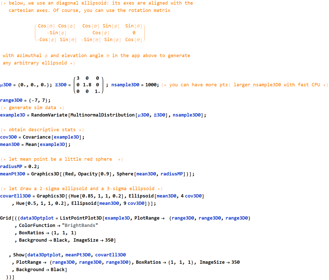
Below is a simple illustration of ellipsoid3D.

code

You can steer it in any direction by moving azimuthal angle φ and elevation angle θ.

Here is an example of 3D normal distribution similar to the above. The code is deliberately shown line by line so that you can follow.

The best way to see your data is to fly through it

code

Here is an example that we will look later: we’ll use height, shouldwidth and chestgirth to distinguish the gender (must execute to read in data - this data is the same as in E .2.0)

Data on human body measurements (open up to see details if needed - but not necessary - just shift+enter)

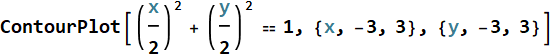
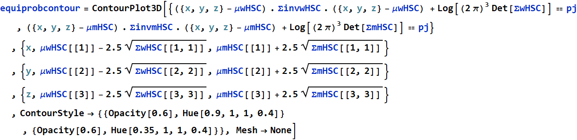
There may be a thing new here that you haven’t learned before: ContourPlot3D and ContourPlot. Both are designed to plot a contour given by an equation or condition. See this example, the contour of function
                                          
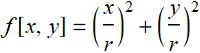
for                                 f[x,y]=positive constant
is the set of {x,y} satisfying that equation, which we know, is a circle:

For a variance ellipsoid:

And for 3D, ContourPlot3D gives a surface, and in the above, we use it to plot the estimated variance ellipsoid of the data.

We can calculate the point along the axis of the two mean points, where the two PDF are equal:

This shows show to discriminate the two clusters. The yellow surface is the Bayes’ decision, it is 50-50% on it and a point belongs to the green cluster if on one side and pink cluster on the other. This is what we will study next.

5. Conditional probability and Bayes’ rule

5.1 Conditional probability

The concept of conditional probability was discussed above for the case of joint distribution men height and shoulder width. For the below, we can make statement such as:
    If a man’s height is between 175-180 cm, then the probability for shoulder width is slice #4:
                       p[shoulder|h∈[175-180] ]=... (slice # 4)

The height is divided into 7 vertical slices as shown. For each slice, we study shoulder width distribution Note the mean of shoulder width (white red dots) increases vs. height

The white line and white/red point mark the mean of the shoulder width in each slice of height. The gray box marks the [+1 standard of deviation, -1 standard of deviation]  interval. Notice that the mean of shoulder width of each slice of height values increases with increasing height. In other words, the shoulder width is correlated with height

Another example: If we want ace of ♠,
               p[ace of ♠] = 1/52

We take a sneak peak and saw this: A
the question now is:  what is the probability that it is A♠, given that we have A? This is how we write it:
                      p[A♠ if A] or p[A♠ | A]

Intuitively, we know our chance is now much better than 1/52:
                  

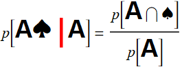
which is 1/2. Likewise, suppose we take a sneak peak and find ♠. There are only 13 cards of spade and one of them is ace, hence:
               

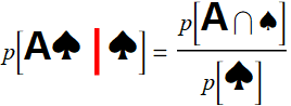
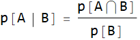
Now we can formally define conditional probability:
                  

Another example: suppose we draw 2 cards, one of it is an ace, what is the probability of having a blackjack? Surely, we must feel better than not knowing what that card is.
Let A: probability of BJ; B: one of the two cards is an ace.
p[A|B]=probability of the other card is a 10:
Use the formula: .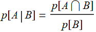
p[A∩B]=p[A]: this is because A is a subset of B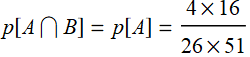
.
p[B]=
Thus: 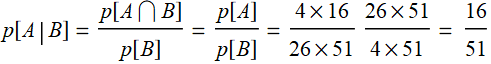, which agrees as above.

5.2 Bayes' rule (theorem) and Bayes’ inference

5.2.1 Bayes’ rule

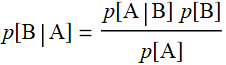
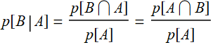Since: and , we have:
                  p[A|B]p[B]=p[B|A]p[A] or:
                        

We will see that the application of Bayes' theorem to do inference is not without ambiguity. It's not just a formula that we can use blindly because there are implicit assumptions that we may overlook. Hence, we should take a step back and think what it means to do inference.

5.2.2 Bayes’ inference

Everyone likes making decision when we have absolute certainty on the information. We face challenge only when the information is ambiguous. We don't have a problem telling the sound from a cat or a dog. A "meow" is pretty distinctive from a "ruff". But there are two dogs, and we are not that familiar with them, whose bark is that?

Bayes’ inference, or Bayesian theory of decision making deals with this type of uncertainty based on Baye’s rule above. In fact, this can be consider as the root of modern day classification algorithms, aka machine learning, machine intelligence. Why do we call “machine intelligence”? Because we think of ourselves as “intelligent” (! :) !!!) and call an algorithm intelligent when it can imitate our hard-wired algorithm in our nervous system that does Bayesian-like inference. If an event, e. g. X has consequence c. When we see “c”, we infer that there may be “X”.

If the pavement and road are wet everywhere, there must have been a rain. This is an inference. Bayesian inference is a quantitative rule to ensure that our inference is quantitatively most rational.

Let’s use this example of US men and women heigth distribution.

This is what you should see from the app.

Suppose a witness sees a person leaving a building. Supposed that the lighting is poor and the sighting is so fleeting that the witness cannot tell if it were a man or a woman. However, the person height is known since he/she was seen to pass under some obstacle of known clearance, such as 63”. We would infer that the person is a woman because after doing the integration, we will find that it is more likely than the probability for a man.

But now someone told us that it was an all-male gathering in that building, would we still make that inference? (assuming that the person has to be one of the people at the gathering). What would be a better inference? A man. With 100% certainty.

Why is it? What changes here? Supposed we know that 90% of attendees were men, only 10% were women, what would be the best guess now? It’s getting difficult isn’t it? A lot of ambiguity. What if the fraction of men is 80% or what if 99%, or 70%, should there be a formula what would be a best guess in each case? Yes, using Bayes’ rule.

Mathematically this is what we need: the probability for a person from that building to be a man or woman AND having height x. The key word here is AND.
1. Let the probability for the person to be a man is p[man], based on the man attendence rate.
Probability for a the person to be a woman is p[woman]=1-p[man].
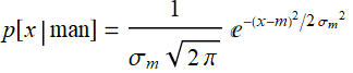
The prob of a person height =x if we know that the person is man is:
                       
Likewise for women: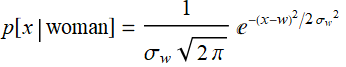     
The probability for a person from that building to be a man AND having height x is:
                                                            p[x,man]=p[x|man] p[man]    
The probability for a person from that building to be a woman AND having height x is:
                                              p[x,woman]=p[x|woman] p[woman]
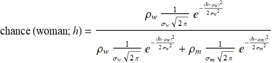
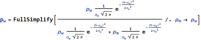
The probability for any person from that building to have a height of  x is:
                               p[x]=p[x|man] p[man]+p[x|woman] p[woman]
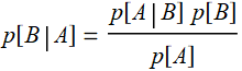
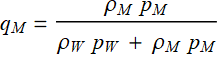
Now we can make an inference: the prob of a person to be a man, given that we know having a height x is:
                                     
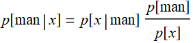
by Bayes' rule. This is the essence of Bayesian inference. The key terms here are p[man] which is prior knowledge of the gathering, and p[x] which is the distribution of the feature we are interested for that sample population.
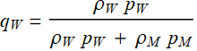
Similarly for woman: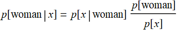    

5.3 Additional examples/exercise

5.3.1 Communication bit-0 and bit-1

5.3.2 Card game

Exercise

Consider the following problem:
Suppose we play a game of in which you will draw 5 cards. The hand is said to be RED or BLACK if a majority of the cards is red or black. You are supposed to bet RED or BLACK. What is the probability for you to have a RED or BLACK hand?
By symmetry of the number of red and black cards, the odd should be 50-50, right?

Supposed you can buy the chance to flip one card open and then bet, for example, you flip one card and find it red. What is the probability for you to have a red hand? Is it still 50%, or better? What would you bet?

The point here is that something changes: it is still the same hand before; but the fact that you know that one card seems to improve your betting chance. Why does the knowledge of one card suddenly change your chance? would you increase your bet? Calculate the probability of winning if you know one card.

Answer

Let B be the event of having a red hand, A: event of one card flipped up is red.

We want to know: p[B|A]. We can use Bayes’ theorem:
                                                     
We need to know p[A|B], which is the probability of one card flipped open is red given that it is a red hand. If it is a red hand, the number of red cards is either 3, 4, or 5. The probability of open one card red is .
Consider “naive Bayes approach”: (not accurate, but useful approximation). Suppose that each possibility above has equal probability, that is 1/3, then the chance for the card flipped to be red, knowing that you have a red hand is: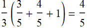
Or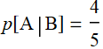                               

What is p[B]? Probability to have a red hand= , hence . What is p[A]? It is the probability to flip up one card red regardless of hand? this is a problem because we don’t really know:
- If all 5 are red, it is 1;
- If all 4 are reds, it is ; and so on, ...
Again, we use naive Bayes approach. Suppose that all 6 possibilities (0,1,2,3,4,5) have equal probability, then                                              
                        

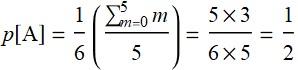
Now, we can put all together:
                            
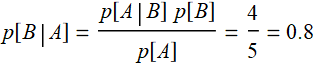
Thus by flipping one card, your chance improves from 0.5 to 0.8: this is a tremendous odd in betting, except that it is not accurate, because the naive Bayes assumption is only a rough guess. We don’t know what are in the card deck: it can be 200 cards, 500 cards with unknown portions of red or black card.

For a 52-card deck, the various terms can be calculated exactly.

Let p[3,4, or 5 cards red], then the probability n red cards for M-card hand is:
                     

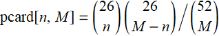
Hence, for a 52-deck, the chance improves from 0.5 to 0.68

code for Monte Carlo sim

Exercise

Let’s say we play with a 52-card deck. The game rule is that one can buy a chance to flip a card with $X (e. g. $100), and after that, one can bet any amount from $0 up to $ q X (e. g. if q=2, q X=$200). If one wins, one gets $ ρ *bet (e. g.  ρ=0.8, the house takes a 20% cut), and if one loses, one loses all of course. Calculate the odd for your strategy. (This is the introduction to the concept of calculation of investment return and market strategy).

Your answer

See supplementary file of Lesson set 6 for answer.

5.3.3 Fair coin

Let’s say we play coin flip games. A fair coin is defined to be 50-50% chance for head and tail. But how do we know if the coin is fair? We do an experiment, flipping it, say 10 times, and get 6 heads, 4 tails. Can we conclude that it’s fair? Or that the probability for head, and that it is not a fair coin?

Clearly, this is not for a cut-and-dry answer. The correct formulation for the answer is that “given the results (6 H, 4 T), the probability for is...” In other words, we can only answer with a probability:
                           ,

Exercise - fair coin analysis

Analyze the problem and calculate  

Answer

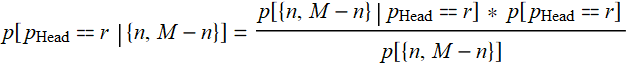
To calculate
            ,
we use Bayes’ theorem:
     

First, we have this result, which is just based on binomial distribution we learn before:
      
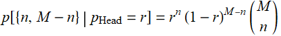
We need:   and p[{n,M-n}].
Here, it is clear that the problem with using Bayes' theorem is that we don't really have any information about   and p[{n,M-n}] without additional assumptions.

First, exactly what means? it means that if we take a coin from a general coin population, which can include all the fair and unfair coins in the world, and test each coin infinite number of times with fair tosses to obtain of each, plot on a PDF histogram and let the population -> ∞, then the histogram PDF will asympotically approaches distribution.

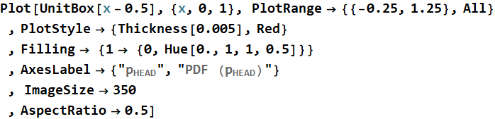
This is the prior probability knowledge that makes Bayes’ theorem ambiguous. In this case, we will just assume that there is no known property of the coin and that the coin bias can range uniformly from 0 (never head, always tail) to 1 (always head, never tail) as illustrated below:

And for p[{n,M-n}]
           

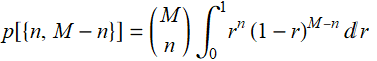
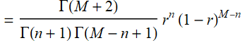
Hence:
    
                                           

code

Discussion

Consider 10 tosses, 5 H, 5T. Is it good enough to declare the coin fair?

The plot above shows us what the chance is for real to be any value from 0-1, knowing that we get (5H,5T) result. We see that the distribution is quite broad. It means that getting 5-5 is not very convincing to say that the coin is really fair.
Let's do it for 100 times. If we get 50-50, what is the chance to have a fair coin now?

Now it looks a bit more convincing. But is it good enough to tell the difference between 0.48 and 0.51? Still not enough. Try it for 1000.

Are we anymore confident to tell 0.501 vs 0.5? Not quite isn't it? This simply shows the nature of statistical deviation. What this mean is that it is not at all easy to measure some small effects without large number of samples.
This is where we get the feeling of "too good to be true". If an experiment comes out too great a result, we don't feel comfortable if the expected statistical fluctuation is not there. Later on, we will see that's where chi-square test and a whole field of searching for outliers come in. It is "statistics" about statistics.

Consider 100 tosses and get 70 heads, 30 tails, can we say anything?

We can say that the ratio of the chance for it to be a fair coin (50-50) vs. a bias coin (70-30) is 0.00027. More precisely, if we get 70 H and 30 T, we can say this:

The probability for the coin to be bias toward head is 99.997%.

6. A numerical exercise on Bayes’ decision with cost

In the following, we will use examples similar to the one below we are already familiar with to review probability

men women Classify the 5 individuals A - E as man or woman, and state the approximate confidence level.

6.1 Demonstration with a game

As mentioned, while we humans can beat spam bots easily with the highly complex calculation task of visual pattern recognition, we aren’t as good as the computer when it comes to even a simplistic numerical calculation.

We can demo with a simple game as shown below:

Take a random adult individual in the US. You are told of his/her height. We can bet that person a man or a woman. If we bet $100 and win, we get $50 pay off. If we lose, we lose the whole $100. Unfair? All casinos must have this “house advantage” to make a living. As usual, there is a cap, a limit how high you can bet. Say $100 max. You don’t have to bet, you can pass if you don’t like the odd. Is that a good game? assuming that the individual is totally random. Do you want to play?

Once you start, you will find out how good you are at probability inference and you would make a fortune until the house escorts you off the premise.

Why? because the odd is very good that you win. But it is meaningless just to win without any benchmark. Beating or at least equal to the computer is the proof-in-pudding of understanding of probability. Let’s start and see what you get. Please follow instructions and do all asked, this is not just a game but it is used to illustrate key points of the lessons.

You can run this game as an independent app - external to the lecture. It is available in the associated App folders along with your lectures. Mathematica is less prone to crash. You can also just copy, cut and paste onto a new notebook. Close or minimize this notebook window while running the app.

Exercise - play game - learn probability inference and loss function

Play against the computer. Here is the info you need to compete against it (no, the computer doesn’t cheat): If you don’t quite understand what the chart below indicates, we have a supplementary topical lecture on normal distribution that you can learn.

Play at least 10 rounds and preferrably more against the computer and record, observe whether you win or lose against the computer. Make an analysis of your performance, study how the computer bets, and derive your strategy. you can click this to see your gamestats vs. computer.
If you can be as good as the computer, then, you understand probability and know normal (Gaussian) distribution well. Explain the theory behind your strategy - which is the optimal approach that the computer uses. If not, it’s OK to continue and we’ll discuss about taking the supplementary topical lecture on normal distribution and probability (go to Course Note page, look inder Supplementary topical lessons).

Be complete in reporting your performance and analyze against computer performance.

Your answer

End exercise of gender height guessing - part 1

Break note: After 6.1, before continuing with 6.2 below, if you need a refresher on Normal distribution and continuous-variable probability, please go either to the supplementary topical lecture or through Section Review Normal distribution below - including doing all exercises (successfully doing the exercises is the only way to confirm the required understanding) - then come back to section 6.2 after you feel confident (with high probability) that you know enough to go on. Otherwise, you might find difficulties in the sections below.

6.2 Probability inference and Bayes’ decision

6.2.1 Basic consideration and exercise

What did you learn from the exercise of playing the game above. How do you classify a person as a man or a woman based on his/her height? How do you think the computer does that? To explore, use the App below

You can run the app below as an independent entity - external to the lecture. It is available in the associated App folders along with your lectures. Mathematica is less prone to crash. You can also just copy, cut and paste onto a new notebook. Close or minimize this notebook window while running the app.

Exercise - basic calculation for Bayes’ decision

Use App Gender height Bayes’ decision above to answer the follow questions:

1- What kind of distribution is your best guess for US men’s and women’s height?
2- What are the mean and variance of each gender distribution based on your visual inspection of the curves. The objective of this question is for you to exercise your visual understanding of normal distribution by guessing approximately the mean and variance directly from the plot. It is not intended for you to be perfectly correct and do not try to spend time to calculate, Internet search, or do anything else. Click “show parm” to check your guesses. Roughly, to within how many % are you correct?
3- Use the app, what is the percentage of women population with height between 57 and 62 in.? what is that value for men?
you can vary the height cursor to the center of 57 and 62, then set the range to 5 inches.
4- What is the percentage of men population with height between 71 and 75 in.? what is the value for women?
5- Apply what you learn about normal distribution, show your calculation by doing integration as shown below to verify the values you obtain from the App. in both Q.3 and Q. 4 above.
                              
for normal distribution, the formula is:    
                  
In Mathematica, erf is Erf.
6- Given a person’s height of 62±0.25 in., how many percent of men with that height and how many percent are women in the general population?
7- Within the narrow selected population of both men and women of that height only, 62±0.25 in., how many percent are men and how many are women (within that population only)? (click on show Bayes’ decision to compare your answer). What is your formula?
8- Do the same as 7 for a person of height 68±0.25 in.
9- Vary the person height in any way you wish, move back and forth, observe the Bayes’ decision (also called Bayesian decision), what is the criterion to decide the person of the given height man or woman?

hidden answer

1- It is evident that both distributions are normal distribution.

2- Using the cursor, the mean for woman is ~ 63.6, SD σ ~ 3”. For men, μ ~ 69.5”, SD σ ~ 3”
The actual values are:
- For women:  μ= 63.6”, the estimate is exact. The SD σ = 2.8”. The estimate is off ~ 0.2/2.8 ~ 7%.
- For men:  μ= 69.2”, the estimate is off by 0.3”, hence: 0.3/70 ~ 4%. The SD σ =3”. The estimate is exact.

3- From the app: the % of women between 57 - 62” is 27.02% and for men: 0.82%

4- From the app: the % of men between 71 - 75” is 24.8% and for women: 0.43%

5- Calculation by using Erf
For women and men between 57 - 62, this is what we do:

For women, surprisingly, the value here: 27.46% is slightly off from Q.3 result: 27.02% the difference is small, but it may mean some error somewhere either in the app or the parameters of the app are not what it says.  
For men, the result 0.817% is in good agreement.
Do the same for Q. 4:

Again, we have excellent agreement with men, 24.77%, while for women, the result here, 0.409% is off from the app: 0.426%. The best guess is that the parameters of women as given in the App may be rounded off with a small difference from the actual values used by the app.

6. Given a person’s height of 62±0.25 in., how many percent of men with that height and how many percent are women in the general population?
The app shows 5.996% of women are of that height range, and 0.375% of men.

7- Within the narrow selected population of both men and women of that height only, 62±0.25 in., how many percent are men and how many are women (within that population only)? (click on show Bayes’ decision to compare your answer). What is your formula?

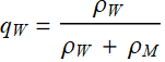
It is quite straight forward. Let’s say the women population of the whole US is: and that of men is , then the population with that height is:
                                          
where and
Then, the percentage of men and women in that population are, respectively:
                             ;       
If the men’s and women’s populations are equal (good approximation but not quite true), then:
                              ;       

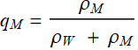Or, 94.1% are women, and 5.9% are men. These values are in good agreement with the Bayes’ decision calculation, showing that Bayes’ calculation implicitly assumes equal women and men population.

8- Do the same as 7 for a person of height 68±0.25 in.

For a person of height 68±0.25 in.:

use the same formula and the same assumption of equal populations:

These proportions of men and women, 74.3% and 25.7% are in good agreement with the Bayes’ decision.

10- Vary the person height in any way you wish, move back and forth, observe the Bayes’ decision (also called Bayesian decision), what is the criterion to decide the person of given height man or woman?

It is obvious that the Bayes’ decision is simple: it decides a man or a woman based on the proportion or probability of man or woman to be >50%.

Exercise - odd and Bayes’ decision - intro to discriminate

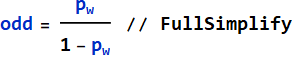
Odd is a very common term - the odd is that you have heard the word “odd,” but exactly what is odd in betting and statistics? Odd is defined as:
                       
This is different from “chance” because chance is probability. In other words:
                                          
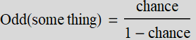
but people are sometimes mistaken chance for odd when the chance is small, because (1-chance) ~ 1 for small chance. In this definition, you can understand the expression “the odd is 1-to-1,” which means the chance is 50-50.
In this exercise, we will examine the quantitative aspect of odd.
1- What is the odd for the person of 68” height to be a man (use the app). Without referring to the app and based on what you get for the odd of a 68” man, what is the odd for a 68” woman? (just ONE simple calculation)

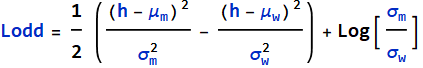
2- If you plot the odd of something vs. the odd against it, which i the odd of not-that-something on a log-log scale, what do you expect?

3- Plot the odd and log(odd) of a woman as a function of height. What is the meaning when log(odd) cross the zero point?

hidden answer

First, let’s assume  

End exercise on basic calculation for Bayes’ decision

6.2.2 Concept of discriminant function

The computer player sets up a threshold, called “discriminant” boundary shown as green line below. One can choose anywhere to set the discriminant line. Then, one can classify any one to the right of that line as man and the left, woman.

As you can see, it doesn’t matter where the discriminant line is, there are always errors: a fraction of women in the red integral will be misclassified as men for being taller than the discriminant height. Likewise, a fraction of men of the blue integral will be misclassified as women for being shorter than the discriminant height.

Move the line to the right, you will make less error on calling “woman” (smaller red integral), but more on “men” (larger blue integral), and vice versa if you move to the left. There is a location for discriminant line that gives a minimum for the sum of both men and women errors, shown as the white dashed line.

Below are plots of the error as a function of the discriminant value.

Exercise - calculation of errors

Write your own code to reproduce the plots of error above. You don’t need to reproduce the style, cursors, markers, etc. Only:
- the curve of misclassified women error (orange above)
- the curve of misclassified women error (blue above)
- the total of both (yellow above)
as a function of the discriminant line location.

Reminder, use Mathematica function Erf or Erfc.

To calculate the error integral, remember this formula:
                  
                  For     b-> ∞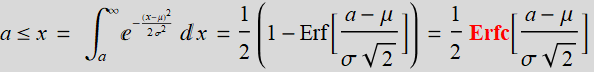                    
                  For a -> -∞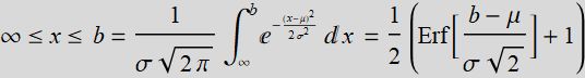               

your answer

Exercise - prove that the minimum total error occurs at the pdf intercept

given answer

The total error is the sum of two things (u is the position of discriminant line):
           category 1 misclassified as cat. 2: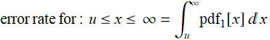  
           cat. 2 misclassified as cat. 1: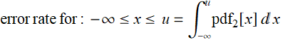          
Total: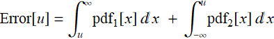                              
The minimum is where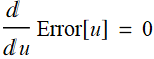                    
Or: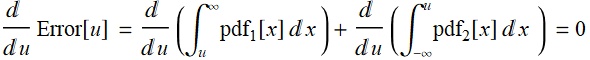                        
which is: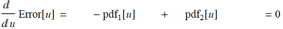               
Hence, the minimum error occurs at:
                                                       
or where the two curves intercept. QED.        

Exercise - calculation of errors in other applications

6.3 Concept of prior distribution and probability

Suppose the game you play above changes a little. Let’s say the person’s height is 68”. The app says:

The odd is almost 3:1 for a man.

But now, instead of a random person of the general US population, that person comes from women’s apparel stores. Do you keep the same guessing strategy, that it is a man, or do you change? Vice versa, consider one more example. Let’s say, a person’s height is 64”.

It appears that the odd is 83-17, or almost 5:1 that it is a woman.

But that random person is from a sport event with 90% being men. Is the odd still 5:1 woman? Let’s put it this way. If we know that sport event is attended by 90% men and we take just a random person, what is the odd of that person a man? it is a 9:1 odd. But now we know that person height. It is 64” should the odd suddenly becomes 5:1 the person is a woman? That doesn’t make any sense!
Or, let’s go to the extreme and say, you have to guess the gender of a person from group that is known to be 100% women or men, is the Bayes’ decision calculation in the App valid? How do we adjust for this?

Let’s step back and consider a simple calculation. Let say sample population of women’s apparel stores customers have 9000 women and 1000 men. Let’s say the person’s height is 68”.

as shown in the left plot, just among men, there is 6.132% of that height. Multiply by 1000, we have:

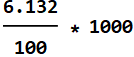
How many women? do the same thing:

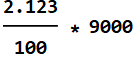
We have 191 women to 61 men of that height from the population who go to women’s apparel stores. Now the probability for a man is only:

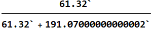
In other words, the odd is 3 to 1 now that it is a woman. This chart:

makes this point. See this:

The slight discrepancy is due to roundoff.

The women population outweights that of men by 9:1 ratio, hence, instead of 3:1 for men if both populations are equal, it flips all around. This is known as prior probability.

women height parameters

Exercise - Bayes’ decision with prior probability on population

You will do a study on how the discriminant boundary (the position of the line that helps make decision on either man or woman) vay as a function of prior probability on population. If you are theoretical in math you can actually derive and plot. Otherwise, you can do this:
- vary the woman population from 0.1 - 0.9
- observed the location of discriminant boundary.
- plot the latter as a function of the former
observe and make your comment, discussion.

your answer

End exercise

6.4 Concept of cost and payoff

Finally, we get to things that matter: cost and payoff. Any statistical calculation in real life, such as financial planning, investment, insurance premium actuary calculation, payoff, etc. boils down to one thing: maximizing return, minimizing loss, lowering or hedging risk. So, we don’t just calculate probability. That’s not complete. It has to be:
         (Probability of event A) x (cost of event A) +   (Probability of event B) x (cost of B) + etc.

If cost is positive, it is a lost. If cost is negative, it is a gain. The objective is to maximize the net return.
If you notice, in the game above, the computer does NOT always put a bet. Why? because the payoff is not 50-50. This is an example what the computer thinks:

               event A: chance to be a man = 60%
If I win:  I get only $50, hence the expected winning is:    60% x $50      =     $30
If I lose, I lose $100.  the expected loss is:                     40% x (- $100)    =   - $40
                                                     net expected return is                              =  - $10
The computer will pass. Why should it play when it expects to lose? In order for it to bet, it requires:
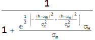
                                                            p × $50-(1-p)×$100 > 0

In other words, it has to be > 0.667 winning probability for it to place a bet and expect a positive return. To the computer, there is NOT one discriminant line, but 2. This is the win-loss curve that the computer looks at:

The above chart shows positive expected payoff in green and loss in red. It will bet if the given height is to the left (bet woman) or the right (bet man) of the two white discriminat lines, but NOT in between the two lines because the expected payoff is negative (red) in that range. That little advantage is why the computer can statistically beat you when playing sufficiently many rounds.
Below is the payoff table. The two curves are simply the two payoff functions in the table for the two strategies: bet woman or bet man for a given height.

So, in a real life practical calculation, the discriminants are calculated based on cost (or payoff) - not a simple Bayes’ decision like what we did above. Supposed the game rule is changed so that if you guess woman wrong, like guessing a woman’s age wrong, you have to pay down double the bet as a penalty, the strategy will be entirely different. Very few will bet on woman and the bet-woman curve will shift further to the left.

The math is still simple, everything is not done with just probability, but as we show above:

         Net (gain/loss) = (Probability of event A) x (cost of event A)   
                                 +   (Probability of event B) x (cost of B)
                                 + etc.

It is the expected return that matters. This is most relevant to investment or financial planning. It is also what insurance actuarians do all the time, from calculating your deductibles to premiums. All to maximize the return (minimizing cost).

Exercise - calculation with cost or payoff

If the game rule changes to this: if the result is a woman, but if you guess it were man, you will lose double of your bet. Everything else the same, what would be your betting strategy. This type of things happen all the time in business when prices change, law/regulation change etc. Companies and business must change how they operate to maintain profit.

your answer

End exercise