Extra materials: Data analysis & Data analytics
ECE 3340 - Han Q. Le (c)
The following materials are for the “breadth-of-knowledge” objective of ECE 3340. They include excerpts from other lectures not necessarily of ECE 3340. Hence, occasional references such as “as discussed previously other lectures” or “from classwork or homework” might not necessarily be related to lectures and/or classwork/homework in ECE 3340.
1. For general knowledge: Recap and general discussion
Excerpt
1.1 General discussion
In the previous lesson, we handle some data and learn some simple approaches to analyze and make use of it. The ultimate goal and use of data processing is to get the information we need and make decision/take action. No matter how complex the data and the processing and calculation is, the ultimate output is quite simple. Consider, for example, the high-stake game of computer trading:

After $M-worth of computing power and software development that digests massive data with lightspeed communication, the outcome is only a few action choices:
- BUY or SHORT COVER (inc. options)
- SELL or SHORT
- HOLD (if already owned)
These are actions that human traders can do on gut feeling or instinct. The good thing though, the computer can’t hide massive trading loss and lie about it like human traders.
The same thing with all other statistical computation: the output is usually discrete or discretized into a few options and choices.
Consider another example: loan application. If someone without a credit score applies for a loan, the first thing is to get one. A credit bureau will run through a calculation of applicant’s financial history (doesn’t matter how complex) to arrive at a single number. That number is further discretized to 5 categories below.
The bottom line is the action: loan approved with certain interest rate: low interest rate for “Excellent” and high for “Fair”, or outright rejection for “Bad” and “Very Bad.”
Below is another example with discrete output:
The following materials are adapted form Netica, a Bayesian Belief Network (BBN) software from Norsys. The example below is from Lauritzen, Steffen L. and David J. Spiegelhalter (1988) "Local computations with probabilities on graphical structures and their application to expert systems" in Journal Royal Statistics Society B, 50(2), 157-194.
We will learn Bayesian Belief Network calculation later, but for now, just consider the example. There are three patients coming to a pulmonary clinic as shown below. Each has certain symptoms, certain test results, may be bloodwork, X-ray etc. This is an example of discrete output: regardless how complex the data and the computation are, the only result that matters is the diagnosis, which in this case can be:
1- if lung cancer
2- if tuberculosis
3- if just bronchitis
The results are discrete outputs 1, 2, 3 as shown above, not some array of continuous real numbers like {25.128, 0.833, ....}.
Although the patients may have similar clinical data (symptoms, test results), they may have different data on other aspects, for example, health history, lifestyle, background, and today, genetic makeup.
Unlike old-fashioned diagnosis that is based only on clinical data, this algorithm takes into account of other data and make decision based on the most probable scenario (maximum likelihood) for each individual Hence, Mr. Smith (case A) and Mr. Doe (case B) both have abnormal chest X-ray but the diagnosis that Mr. Smith is more likely to have tuberculosis while Mr. Doe is more likely to have cancer. Ms. Andrews is luckier as she most likely just have bronchitis.
We will learn this stuff later. The bottom line is, a lot of time, human actions require things to be discretized into a small number of choices.

1.2 Review of cluster analysis concepts
We discuss concepts “clustering” and “classification” last lesson. In light of the discussion above, cluster analysis - similarly to the example of pulmonary disease diagnosis, is simply a statistical calculation with discrete output: the designation of clusters - which and which - are the output. More precisely, the properties or responses associated with the clusters are the output of interest.
Let’s review the key ideas from the last lesson:
1. Data sometimes can be grouped into distinctive clusters based on “features” that are characteristic to each cluster, and can be used to discriminate the clusters from each other. (By default, there must be at least 2 clusters: the one of interest, and the rest that is not that one. Usually, there are more than these two basic ones). Finding the crucial features is a key task.
2. Given a new data point, the objective is to use the features of that data to classify which cluster it belongs to. Of course, there is a possibility that it doesn’t seem to belong to any existing cluster, then it may indicate a new cluster.
3- We can determine or predict the response (or properties) of the entity associated with the new data point based on the known cluster’s characteristic responses and properties.
An analogy is when biologists encounter a new animal hitherto unknown. The biologists must classify the animal as belonging to a certain extant species, or representing a new species (a new cluster that is distinctive to all known clusters). Then, the new species must be determined if it belongs to some known genus. If not, may be a new genus, or new family and so on.
By classifying a data point to a cluster, like a new species animal to its genus, we can make a prediction of its properties and behaviors based on known characteristics of that genus. (Of course, it can be wrong. If the Giant Panda were newly discovered, no one would blame the discoverer to run for his/her life like running away from a grizzly or a polar bear - which tends to be futile anyway).
In order to do classification, we must have pattern recognition. In fact, this is what we do all the time because we humans are pretty good at it, as shown in the follow.
1.3 Examples of pattern recognition and classification
We humans are actually very good at doing certain task of pattern recognition and classification. As an example, consider this:
It is a raging battle on the Internet as websites try to correctly classify human users from spam bots. The most common method is to use a feature that is very characteristic of human to discriminate against spam bots: the human’s keen ability of visual classification. In this example, a user is asked to do a classification task:
This method itself is to serve as a classifier: to classify the user as human or spam bot. The premise of the method is that a human will be better and make far less errors than spam bots, and hence, it uses this feature: correct classification to determine if a user is a human or not.
Exercise
In this exercise, for each captcha image, like the one illustrated above, you must identify: the clusters (e. g. food and non-food), how many data points, and what features you think a user must use to classify correctly. Imagine how to write a code to teach a computer to identify a sandwich (last image) but pizza is not a sandwich. What features that make a sandwich a sandwich? (think of the expression “I was sandwiched in the middle seat between two oversized people who spilled their bodies over the armrests during the entire flight...”)
![Graphics:PlotLabel /. Options[{RowBox[{RowBox[{GraphicsBox[TagBox[RasterBox[NumericArray[<458,305,3>, UnsignedInteger8], {{0, 458}, {305, 0}}, {0, 255}, ColorFunction -> RGBColor], BoxForm`ImageTag[System`Convert`CommonDump`ConvertText[Byte, System`Convert`HTMLDump`htmlsave, HTMLEntities -> {HTMLBasic}, AltMathOutput -> PlotLabel, WindowSize -> {2000, Automatic}, MathOutput -> PNG, ConvertClosed -> False, ConvertReverseClosed -> False, ConvertLinkedNotebooks -> False, CharacterEncoding -> Automatic, ConversionStyleEnvironment -> None, ConversionRules -> Automatic, HeadAttributes -> {}, HeadElements -> {}, CSS -> Automatic, ConvertLinkedNotebooks -> False, MathOutput -> GIF, GraphicsOutput -> GIF, Graphics3DOutput -> Automatic, ManipulateOutput -> CDF, ConvertClosed -> True, ConvertReverseClosed -> False, FullDocument -> True, AltMathOutput -> FileName, TableOutput -> {TextForm, Automatic}, AnimationOutput -> Automatic, FilesDirectory -> HTMLFiles, LinksDirectory -> HTMLLinks, HTMLEntities -> {HTML}, AllowBlockMathML -> False, ShowStyles -> True, DataUri -> False, MathMLOptions -> {UseUnicodePlane1Characters -> False, IncludeMarkupAnnotations -> False, Entities -> MathML}], ColorSpace -> System`Convert`CommonDump`ConvertText[RGB, System`Convert`HTMLDump`htmlsave, HTMLEntities -> {HTMLBasic}, AltMathOutput -> PlotLabel, WindowSize -> {2000, Automatic}, MathOutput -> PNG, ConvertClosed -> False, ConvertReverseClosed -> False, ConvertLinkedNotebooks -> False, CharacterEncoding -> Automatic, ConversionStyleEnvironment -> None, ConversionRules -> Automatic, HeadAttributes -> {}, HeadElements -> {}, CSS -> Automatic, ConvertLinkedNotebooks -> False, MathOutput -> GIF, GraphicsOutput -> GIF, Graphics3DOutput -> Automatic, ManipulateOutput -> CDF, ConvertClosed -> True, ConvertReverseClosed -> False, FullDocument -> True, AltMathOutput -> FileName, TableOutput -> {TextForm, Automatic}, AnimationOutput -> Automatic, FilesDirectory -> HTMLFiles, LinksDirectory -> HTMLLinks, HTMLEntities -> {HTML}, AllowBlockMathML -> False, ShowStyles -> True, DataUri -> False, MathMLOptions -> {UseUnicodePlane1Characters -> False, IncludeMarkupAnnotations -> False, Entities -> MathML}], Interleaving -> True], Selectable -> False], DefaultBaseStyle -> System`Convert`CommonDump`ConvertText[ImageGraphics, System`Convert`HTMLDump`htmlsave, HTMLEntities -> {HTMLBasic}, AltMathOutput -> PlotLabel, WindowSize -> {2000, Automatic}, MathOutput -> PNG, ConvertClosed -> False, ConvertReverseClosed -> False, ConvertLinkedNotebooks -> False, CharacterEncoding -> Automatic, ConversionStyleEnvironment -> None, ConversionRules -> Automatic, HeadAttributes -> {}, HeadElements -> {}, CSS -> Automatic, ConvertLinkedNotebooks -> False, MathOutput -> GIF, GraphicsOutput -> GIF, Graphics3DOutput -> Automatic, ManipulateOutput -> CDF, ConvertClosed -> True, ConvertReverseClosed -> False, FullDocument -> True, AltMathOutput -> FileName, TableOutput -> {TextForm, Automatic}, AnimationOutput -> Automatic, FilesDirectory -> HTMLFiles, LinksDirectory -> HTMLLinks, HTMLEntities -> {HTML}, AllowBlockMathML -> False, ShowStyles -> True, DataUri -> False, MathMLOptions -> {UseUnicodePlane1Characters -> False, IncludeMarkupAnnotations -> False, Entities -> MathML}], ImageSize -> {273.487, Automatic}, ImageSizeRaw -> {305, 458}, PlotRange -> {{0, 305}, {0, 458}}], , GraphicsBox[TagBox[RasterBox[NumericArray[<606,402,4>, UnsignedInteger8], {{0, 606}, {402, 0}}, {0, 255}, ColorFunction -> RGBColor], BoxForm`ImageTag[System`Convert`CommonDump`ConvertText[Byte, System`Convert`HTMLDump`htmlsave, HTMLEntities -> {HTMLBasic}, AltMathOutput -> PlotLabel, WindowSize -> {2000, Automatic}, MathOutput -> PNG, ConvertClosed -> False, ConvertReverseClosed -> False, ConvertLinkedNotebooks -> False, CharacterEncoding -> Automatic, ConversionStyleEnvironment -> None, ConversionRules -> Automatic, HeadAttributes -> {}, HeadElements -> {}, CSS -> Automatic, ConvertLinkedNotebooks -> False, MathOutput -> GIF, GraphicsOutput -> GIF, Graphics3DOutput -> Automatic, ManipulateOutput -> CDF, ConvertClosed -> True, ConvertReverseClosed -> False, FullDocument -> True, AltMathOutput -> FileName, TableOutput -> {TextForm, Automatic}, AnimationOutput -> Automatic, FilesDirectory -> HTMLFiles, LinksDirectory -> HTMLLinks, HTMLEntities -> {HTML}, AllowBlockMathML -> False, ShowStyles -> True, DataUri -> False, MathMLOptions -> {UseUnicodePlane1Characters -> False, IncludeMarkupAnnotations -> False, Entities -> MathML}], ColorSpace -> ColorProfileData[NumericArray[<3892>, UnsignedInteger8], System`Convert`CommonDump`ConvertText[RGB, System`Convert`HTMLDump`htmlsave, HTMLEntities -> {HTMLBasic}, AltMathOutput -> PlotLabel, WindowSize -> {2000, Automatic}, MathOutput -> PNG, ConvertClosed -> False, ConvertReverseClosed -> False, ConvertLinkedNotebooks -> False, CharacterEncoding -> Automatic, ConversionStyleEnvironment -> None, ConversionRules -> Automatic, HeadAttributes -> {}, HeadElements -> {}, CSS -> Automatic, ConvertLinkedNotebooks -> False, MathOutput -> GIF, GraphicsOutput -> GIF, Graphics3DOutput -> Automatic, ManipulateOutput -> CDF, ConvertClosed -> True, ConvertReverseClosed -> False, FullDocument -> True, AltMathOutput -> FileName, TableOutput -> {TextForm, Automatic}, AnimationOutput -> Automatic, FilesDirectory -> HTMLFiles, LinksDirectory -> HTMLLinks, HTMLEntities -> {HTML}, AllowBlockMathML -> False, ShowStyles -> True, DataUri -> False, MathMLOptions -> {UseUnicodePlane1Characters -> False, IncludeMarkupAnnotations -> False, Entities -> MathML}], System`Convert`CommonDump`ConvertText[XYZ, System`Convert`HTMLDump`htmlsave, HTMLEntities -> {HTMLBasic}, AltMathOutput -> PlotLabel, WindowSize -> {2000, Automatic}, MathOutput -> PNG, ConvertClosed -> False, ConvertReverseClosed -> False, ConvertLinkedNotebooks -> False, CharacterEncoding -> Automatic, ConversionStyleEnvironment -> None, ConversionRules -> Automatic, HeadAttributes -> {}, HeadElements -> {}, CSS -> Automatic, ConvertLinkedNotebooks -> False, MathOutput -> GIF, GraphicsOutput -> GIF, Graphics3DOutput -> Automatic, ManipulateOutput -> CDF, ConvertClosed -> True, ConvertReverseClosed -> False, FullDocument -> True, AltMathOutput -> FileName, TableOutput -> {TextForm, Automatic}, AnimationOutput -> Automatic, FilesDirectory -> HTMLFiles, LinksDirectory -> HTMLLinks, HTMLEntities -> {HTML}, AllowBlockMathML -> False, ShowStyles -> True, DataUri -> False, MathMLOptions -> {UseUnicodePlane1Characters -> False, IncludeMarkupAnnotations -> False, Entities -> MathML}]], Interleaving -> True, MetaInformation -> Association[System`Convert`CommonDump`ConvertText[Comments, System`Convert`HTMLDump`htmlsave, HTMLEntities -> {HTMLBasic}, AltMathOutput -> PlotLabel, WindowSize -> {2000, Automatic}, MathOutput -> PNG, ConvertClosed -> False, ConvertReverseClosed -> False, ConvertLinkedNotebooks -> False, CharacterEncoding -> Automatic, ConversionStyleEnvironment -> None, ConversionRules -> Automatic, HeadAttributes -> {}, HeadElements -> {}, CSS -> Automatic, ConvertLinkedNotebooks -> False, MathOutput -> GIF, GraphicsOutput -> GIF, Graphics3DOutput -> Automatic, ManipulateOutput -> CDF, ConvertClosed -> True, ConvertReverseClosed -> False, FullDocument -> True, AltMathOutput -> FileName, TableOutput -> {TextForm, Automatic}, AnimationOutput -> Automatic, FilesDirectory -> HTMLFiles, LinksDirectory -> HTMLLinks, HTMLEntities -> {HTML}, AllowBlockMathML -> False, ShowStyles -> True, DataUri -> False, MathMLOptions -> {UseUnicodePlane1Characters -> False, IncludeMarkupAnnotations -> False, Entities -> MathML}] -> Association[System`Convert`CommonDump`ConvertText[XML:com.adobe.xmp, System`Convert`HTMLDump`htmlsave, HTMLEntities -> {HTMLBasic}, AltMathOutput -> PlotLabel, WindowSize -> {2000, Automatic}, MathOutput -> PNG, ConvertClosed -> False, ConvertReverseClosed -> False, ConvertLinkedNotebooks -> False, CharacterEncoding -> Automatic, ConversionStyleEnvironment -> None, ConversionRules -> Automatic, HeadAttributes -> {}, HeadElements -> {}, CSS -> Automatic, ConvertLinkedNotebooks -> False, MathOutput -> GIF, GraphicsOutput -> GIF, Graphics3DOutput -> Automatic, ManipulateOutput -> CDF, ConvertClosed -> True, ConvertReverseClosed -> False, FullDocument -> True, AltMathOutput -> FileName, TableOutput -> {TextForm, Automatic}, AnimationOutput -> Automatic, FilesDirectory -> HTMLFiles, LinksDirectory -> HTMLLinks, HTMLEntities -> {HTML}, AllowBlockMathML -> False, ShowStyles -> True, DataUri -> False, MathMLOptions -> {UseUnicodePlane1Characters -> False, IncludeMarkupAnnotations -> False, Entities -> MathML}] -> System`Convert`CommonDump`ConvertText[<x:xmpmeta xmlns:x=adobe:ns:meta/ x:xmptk=XMP Core 5.4.0> <rdf:RDF xmlns:rdf=http://www.w3.org/1999/02/22-rdf-syntax-ns#><rdf:Description rdf:about=xmlns:exif=http://ns.adobe.com/exif/1.0/> <exif:PixelXDimension>804</exif:PixelXDimension> <exif:PixelYDimension>1212</exif:PixelYDimension></rdf:Description> </rdf:RDF></x:xmpmeta>, System`Convert`HTMLDump`htmlsave, HTMLEntities -> {HTMLBasic}, AltMathOutput -> PlotLabel, WindowSize -> {2000, Automatic}, MathOutput -> PNG, ConvertClosed -> False, ConvertReverseClosed -> False, ConvertLinkedNotebooks -> False, CharacterEncoding -> Automatic, ConversionStyleEnvironment -> None, ConversionRules -> Automatic, HeadAttributes -> {}, HeadElements -> {}, CSS -> Automatic, ConvertLinkedNotebooks -> False, MathOutput -> GIF, GraphicsOutput -> GIF, Graphics3DOutput -> Automatic, ManipulateOutput -> CDF, ConvertClosed -> True, ConvertReverseClosed -> False, FullDocument -> True, AltMathOutput -> FileName, TableOutput -> {TextForm, Automatic}, AnimationOutput -> Automatic, FilesDirectory -> HTMLFiles, LinksDirectory -> HTMLLinks, HTMLEntities -> {HTML}, AllowBlockMathML -> False, ShowStyles -> True, DataUri -> False, MathMLOptions -> {UseUnicodePlane1Characters -> False, IncludeMarkupAnnotations -> False, Entities -> MathML}]]]], Selectable -> False], DefaultBaseStyle -> System`Convert`CommonDump`ConvertText[ImageGraphics, System`Convert`HTMLDump`htmlsave, HTMLEntities -> {HTMLBasic}, AltMathOutput -> PlotLabel, WindowSize -> {2000, Automatic}, MathOutput -> PNG, ConvertClosed -> False, ConvertReverseClosed -> False, ConvertLinkedNotebooks -> False, CharacterEncoding -> Automatic, ConversionStyleEnvironment -> None, ConversionRules -> Automatic, HeadAttributes -> {}, HeadElements -> {}, CSS -> Automatic, ConvertLinkedNotebooks -> False, MathOutput -> GIF, GraphicsOutput -> GIF, Graphics3DOutput -> Automatic, ManipulateOutput -> CDF, ConvertClosed -> True, ConvertReverseClosed -> False, FullDocument -> True, AltMathOutput -> FileName, TableOutput -> {TextForm, Automatic}, AnimationOutput -> Automatic, FilesDirectory -> HTMLFiles, LinksDirectory -> HTMLLinks, HTMLEntities -> {HTML}, AllowBlockMathML -> False, ShowStyles -> True, DataUri -> False, MathMLOptions -> {UseUnicodePlane1Characters -> False, IncludeMarkupAnnotations -> False, Entities -> MathML}], ImageSize -> {256.991, Automatic}, ImageSizeRaw -> {402, 606}, PlotRange -> {{0, 402}, {0, 606}}], , GraphicsBox[TagBox[RasterBox[NumericArray[<876,500,3>, UnsignedInteger8], {{0, 876}, {500, 0}}, {0, 255}, ColorFunction -> RGBColor], BoxForm`ImageTag[System`Convert`CommonDump`ConvertText[Byte, System`Convert`HTMLDump`htmlsave, HTMLEntities -> {HTMLBasic}, AltMathOutput -> PlotLabel, WindowSize -> {2000, Automatic}, MathOutput -> PNG, ConvertClosed -> False, ConvertReverseClosed -> False, ConvertLinkedNotebooks -> False, CharacterEncoding -> Automatic, ConversionStyleEnvironment -> None, ConversionRules -> Automatic, HeadAttributes -> {}, HeadElements -> {}, CSS -> Automatic, ConvertLinkedNotebooks -> False, MathOutput -> GIF, GraphicsOutput -> GIF, Graphics3DOutput -> Automatic, ManipulateOutput -> CDF, ConvertClosed -> True, ConvertReverseClosed -> False, FullDocument -> True, AltMathOutput -> FileName, TableOutput -> {TextForm, Automatic}, AnimationOutput -> Automatic, FilesDirectory -> HTMLFiles, LinksDirectory -> HTMLLinks, HTMLEntities -> {HTML}, AllowBlockMathML -> False, ShowStyles -> True, DataUri -> False, MathMLOptions -> {UseUnicodePlane1Characters -> False, IncludeMarkupAnnotations -> False, Entities -> MathML}], ColorSpace -> System`Convert`CommonDump`ConvertText[RGB, System`Convert`HTMLDump`htmlsave, HTMLEntities -> {HTMLBasic}, AltMathOutput -> PlotLabel, WindowSize -> {2000, Automatic}, MathOutput -> PNG, ConvertClosed -> False, ConvertReverseClosed -> False, ConvertLinkedNotebooks -> False, CharacterEncoding -> Automatic, ConversionStyleEnvironment -> None, ConversionRules -> Automatic, HeadAttributes -> {}, HeadElements -> {}, CSS -> Automatic, ConvertLinkedNotebooks -> False, MathOutput -> GIF, GraphicsOutput -> GIF, Graphics3DOutput -> Automatic, ManipulateOutput -> CDF, ConvertClosed -> True, ConvertReverseClosed -> False, FullDocument -> True, AltMathOutput -> FileName, TableOutput -> {TextForm, Automatic}, AnimationOutput -> Automatic, FilesDirectory -> HTMLFiles, LinksDirectory -> HTMLLinks, HTMLEntities -> {HTML}, AllowBlockMathML -> False, ShowStyles -> True, DataUri -> False, MathMLOptions -> {UseUnicodePlane1Characters -> False, IncludeMarkupAnnotations -> False, Entities -> MathML}], Interleaving -> True], Selectable -> False], DefaultBaseStyle -> System`Convert`CommonDump`ConvertText[ImageGraphics, System`Convert`HTMLDump`htmlsave, HTMLEntities -> {HTMLBasic}, AltMathOutput -> PlotLabel, WindowSize -> {2000, Automatic}, MathOutput -> PNG, ConvertClosed -> False, ConvertReverseClosed -> False, ConvertLinkedNotebooks -> False, CharacterEncoding -> Automatic, ConversionStyleEnvironment -> None, ConversionRules -> Automatic, HeadAttributes -> {}, HeadElements -> {}, CSS -> Automatic, ConvertLinkedNotebooks -> False, MathOutput -> GIF, GraphicsOutput -> GIF, Graphics3DOutput -> Automatic, ManipulateOutput -> CDF, ConvertClosed -> True, ConvertReverseClosed -> False, FullDocument -> True, AltMathOutput -> FileName, TableOutput -> {TextForm, Automatic}, AnimationOutput -> Automatic, FilesDirectory -> HTMLFiles, LinksDirectory -> HTMLLinks, HTMLEntities -> {HTML}, AllowBlockMathML -> False, ShowStyles -> True, DataUri -> False, MathMLOptions -> {UseUnicodePlane1Characters -> False, IncludeMarkupAnnotations -> False, Entities -> MathML}], ImageSize -> {216.87, Automatic}, ImageSizeRaw -> {500, 876}, PlotRange -> {{0, 500}, {0, 876}}]}], }], , RowBox[{GraphicsBox[TagBox[RasterBox[NumericArray[<1144,727,3>, UnsignedInteger8], {{0, 1144}, {727, 0}}, {0, 255}, ColorFunction -> RGBColor], BoxForm`ImageTag[System`Convert`CommonDump`ConvertText[Byte, System`Convert`HTMLDump`htmlsave, HTMLEntities -> {HTMLBasic}, AltMathOutput -> PlotLabel, WindowSize -> {2000, Automatic}, MathOutput -> PNG, ConvertClosed -> False, ConvertReverseClosed -> False, ConvertLinkedNotebooks -> False, CharacterEncoding -> Automatic, ConversionStyleEnvironment -> None, ConversionRules -> Automatic, HeadAttributes -> {}, HeadElements -> {}, CSS -> Automatic, ConvertLinkedNotebooks -> False, MathOutput -> GIF, GraphicsOutput -> GIF, Graphics3DOutput -> Automatic, ManipulateOutput -> CDF, ConvertClosed -> True, ConvertReverseClosed -> False, FullDocument -> True, AltMathOutput -> FileName, TableOutput -> {TextForm, Automatic}, AnimationOutput -> Automatic, FilesDirectory -> HTMLFiles, LinksDirectory -> HTMLLinks, HTMLEntities -> {HTML}, AllowBlockMathML -> False, ShowStyles -> True, DataUri -> False, MathMLOptions -> {UseUnicodePlane1Characters -> False, IncludeMarkupAnnotations -> False, Entities -> MathML}], ColorSpace -> System`Convert`CommonDump`ConvertText[RGB, System`Convert`HTMLDump`htmlsave, HTMLEntities -> {HTMLBasic}, AltMathOutput -> PlotLabel, WindowSize -> {2000, Automatic}, MathOutput -> PNG, ConvertClosed -> False, ConvertReverseClosed -> False, ConvertLinkedNotebooks -> False, CharacterEncoding -> Automatic, ConversionStyleEnvironment -> None, ConversionRules -> Automatic, HeadAttributes -> {}, HeadElements -> {}, CSS -> Automatic, ConvertLinkedNotebooks -> False, MathOutput -> GIF, GraphicsOutput -> GIF, Graphics3DOutput -> Automatic, ManipulateOutput -> CDF, ConvertClosed -> True, ConvertReverseClosed -> False, FullDocument -> True, AltMathOutput -> FileName, TableOutput -> {TextForm, Automatic}, AnimationOutput -> Automatic, FilesDirectory -> HTMLFiles, LinksDirectory -> HTMLLinks, HTMLEntities -> {HTML}, AllowBlockMathML -> False, ShowStyles -> True, DataUri -> False, MathMLOptions -> {UseUnicodePlane1Characters -> False, IncludeMarkupAnnotations -> False, Entities -> MathML}], Interleaving -> True], Selectable -> False], DefaultBaseStyle -> System`Convert`CommonDump`ConvertText[ImageGraphics, System`Convert`HTMLDump`htmlsave, HTMLEntities -> {HTMLBasic}, AltMathOutput -> PlotLabel, WindowSize -> {2000, Automatic}, MathOutput -> PNG, ConvertClosed -> False, ConvertReverseClosed -> False, ConvertLinkedNotebooks -> False, CharacterEncoding -> Automatic, ConversionStyleEnvironment -> None, ConversionRules -> Automatic, HeadAttributes -> {}, HeadElements -> {}, CSS -> Automatic, ConvertLinkedNotebooks -> False, MathOutput -> GIF, GraphicsOutput -> GIF, Graphics3DOutput -> Automatic, ManipulateOutput -> CDF, ConvertClosed -> True, ConvertReverseClosed -> False, FullDocument -> True, AltMathOutput -> FileName, TableOutput -> {TextForm, Automatic}, AnimationOutput -> Automatic, FilesDirectory -> HTMLFiles, LinksDirectory -> HTMLLinks, HTMLEntities -> {HTML}, AllowBlockMathML -> False, ShowStyles -> True, DataUri -> False, MathMLOptions -> {UseUnicodePlane1Characters -> False, IncludeMarkupAnnotations -> False, Entities -> MathML}], ImageSize -> {242.024, Automatic}, ImageSizeRaw -> {727, 1144}, PlotRange -> {{0, 727}, {0, 1144}}], , GraphicsBox[TagBox[RasterBox[NumericArray[<1146,796,3>, UnsignedInteger8], {{0, 1146}, {796, 0}}, {0, 255}, ColorFunction -> RGBColor], BoxForm`ImageTag[System`Convert`CommonDump`ConvertText[Byte, System`Convert`HTMLDump`htmlsave, HTMLEntities -> {HTMLBasic}, AltMathOutput -> PlotLabel, WindowSize -> {2000, Automatic}, MathOutput -> PNG, ConvertClosed -> False, ConvertReverseClosed -> False, ConvertLinkedNotebooks -> False, CharacterEncoding -> Automatic, ConversionStyleEnvironment -> None, ConversionRules -> Automatic, HeadAttributes -> {}, HeadElements -> {}, CSS -> Automatic, ConvertLinkedNotebooks -> False, MathOutput -> GIF, GraphicsOutput -> GIF, Graphics3DOutput -> Automatic, ManipulateOutput -> CDF, ConvertClosed -> True, ConvertReverseClosed -> False, FullDocument -> True, AltMathOutput -> FileName, TableOutput -> {TextForm, Automatic}, AnimationOutput -> Automatic, FilesDirectory -> HTMLFiles, LinksDirectory -> HTMLLinks, HTMLEntities -> {HTML}, AllowBlockMathML -> False, ShowStyles -> True, DataUri -> False, MathMLOptions -> {UseUnicodePlane1Characters -> False, IncludeMarkupAnnotations -> False, Entities -> MathML}], ColorSpace -> System`Convert`CommonDump`ConvertText[RGB, System`Convert`HTMLDump`htmlsave, HTMLEntities -> {HTMLBasic}, AltMathOutput -> PlotLabel, WindowSize -> {2000, Automatic}, MathOutput -> PNG, ConvertClosed -> False, ConvertReverseClosed -> False, ConvertLinkedNotebooks -> False, CharacterEncoding -> Automatic, ConversionStyleEnvironment -> None, ConversionRules -> Automatic, HeadAttributes -> {}, HeadElements -> {}, CSS -> Automatic, ConvertLinkedNotebooks -> False, MathOutput -> GIF, GraphicsOutput -> GIF, Graphics3DOutput -> Automatic, ManipulateOutput -> CDF, ConvertClosed -> True, ConvertReverseClosed -> False, FullDocument -> True, AltMathOutput -> FileName, TableOutput -> {TextForm, Automatic}, AnimationOutput -> Automatic, FilesDirectory -> HTMLFiles, LinksDirectory -> HTMLLinks, HTMLEntities -> {HTML}, AllowBlockMathML -> False, ShowStyles -> True, DataUri -> False, MathMLOptions -> {UseUnicodePlane1Characters -> False, IncludeMarkupAnnotations -> False, Entities -> MathML}], Interleaving -> True], Selectable -> False], DefaultBaseStyle -> System`Convert`CommonDump`ConvertText[ImageGraphics, System`Convert`HTMLDump`htmlsave, HTMLEntities -> {HTMLBasic}, AltMathOutput -> PlotLabel, WindowSize -> {2000, Automatic}, MathOutput -> PNG, ConvertClosed -> False, ConvertReverseClosed -> False, ConvertLinkedNotebooks -> False, CharacterEncoding -> Automatic, ConversionStyleEnvironment -> None, ConversionRules -> Automatic, HeadAttributes -> {}, HeadElements -> {}, CSS -> Automatic, ConvertLinkedNotebooks -> False, MathOutput -> GIF, GraphicsOutput -> GIF, Graphics3DOutput -> Automatic, ManipulateOutput -> CDF, ConvertClosed -> True, ConvertReverseClosed -> False, FullDocument -> True, AltMathOutput -> FileName, TableOutput -> {TextForm, Automatic}, AnimationOutput -> Automatic, FilesDirectory -> HTMLFiles, LinksDirectory -> HTMLLinks, HTMLEntities -> {HTML}, AllowBlockMathML -> False, ShowStyles -> True, DataUri -> False, MathMLOptions -> {UseUnicodePlane1Characters -> False, IncludeMarkupAnnotations -> False, Entities -> MathML}], ImageSize -> {271.233, Automatic}, ImageSizeRaw -> {796, 1146}, PlotRange -> {{0, 796}, {0, 1146}}], , GraphicsBox[TagBox[RasterBox[NumericArray[<641,442,3>, UnsignedInteger8], {{0, 641}, {442, 0}}, {0, 255}, ColorFunction -> RGBColor], BoxForm`ImageTag[System`Convert`CommonDump`ConvertText[Byte, System`Convert`HTMLDump`htmlsave, HTMLEntities -> {HTMLBasic}, AltMathOutput -> PlotLabel, WindowSize -> {2000, Automatic}, MathOutput -> PNG, ConvertClosed -> False, ConvertReverseClosed -> False, ConvertLinkedNotebooks -> False, CharacterEncoding -> Automatic, ConversionStyleEnvironment -> None, ConversionRules -> Automatic, HeadAttributes -> {}, HeadElements -> {}, CSS -> Automatic, ConvertLinkedNotebooks -> False, MathOutput -> GIF, GraphicsOutput -> GIF, Graphics3DOutput -> Automatic, ManipulateOutput -> CDF, ConvertClosed -> True, ConvertReverseClosed -> False, FullDocument -> True, AltMathOutput -> FileName, TableOutput -> {TextForm, Automatic}, AnimationOutput -> Automatic, FilesDirectory -> HTMLFiles, LinksDirectory -> HTMLLinks, HTMLEntities -> {HTML}, AllowBlockMathML -> False, ShowStyles -> True, DataUri -> False, MathMLOptions -> {UseUnicodePlane1Characters -> False, IncludeMarkupAnnotations -> False, Entities -> MathML}], ColorSpace -> ColorProfileData[NumericArray[<6936>, UnsignedInteger8], System`Convert`CommonDump`ConvertText[RGB, System`Convert`HTMLDump`htmlsave, HTMLEntities -> {HTMLBasic}, AltMathOutput -> PlotLabel, WindowSize -> {2000, Automatic}, MathOutput -> PNG, ConvertClosed -> False, ConvertReverseClosed -> False, ConvertLinkedNotebooks -> False, CharacterEncoding -> Automatic, ConversionStyleEnvironment -> None, ConversionRules -> Automatic, HeadAttributes -> {}, HeadElements -> {}, CSS -> Automatic, ConvertLinkedNotebooks -> False, MathOutput -> GIF, GraphicsOutput -> GIF, Graphics3DOutput -> Automatic, ManipulateOutput -> CDF, ConvertClosed -> True, ConvertReverseClosed -> False, FullDocument -> True, AltMathOutput -> FileName, TableOutput -> {TextForm, Automatic}, AnimationOutput -> Automatic, FilesDirectory -> HTMLFiles, LinksDirectory -> HTMLLinks, HTMLEntities -> {HTML}, AllowBlockMathML -> False, ShowStyles -> True, DataUri -> False, MathMLOptions -> {UseUnicodePlane1Characters -> False, IncludeMarkupAnnotations -> False, Entities -> MathML}], System`Convert`CommonDump`ConvertText[XYZ, System`Convert`HTMLDump`htmlsave, HTMLEntities -> {HTMLBasic}, AltMathOutput -> PlotLabel, WindowSize -> {2000, Automatic}, MathOutput -> PNG, ConvertClosed -> False, ConvertReverseClosed -> False, ConvertLinkedNotebooks -> False, CharacterEncoding -> Automatic, ConversionStyleEnvironment -> None, ConversionRules -> Automatic, HeadAttributes -> {}, HeadElements -> {}, CSS -> Automatic, ConvertLinkedNotebooks -> False, MathOutput -> GIF, GraphicsOutput -> GIF, Graphics3DOutput -> Automatic, ManipulateOutput -> CDF, ConvertClosed -> True, ConvertReverseClosed -> False, FullDocument -> True, AltMathOutput -> FileName, TableOutput -> {TextForm, Automatic}, AnimationOutput -> Automatic, FilesDirectory -> HTMLFiles, LinksDirectory -> HTMLLinks, HTMLEntities -> {HTML}, AllowBlockMathML -> False, ShowStyles -> True, DataUri -> False, MathMLOptions -> {UseUnicodePlane1Characters -> False, IncludeMarkupAnnotations -> False, Entities -> MathML}]], ImageResolution -> {72, 72}, Interleaving -> True, MetaInformation -> Association[System`Convert`CommonDump`ConvertText[Exif, System`Convert`HTMLDump`htmlsave, HTMLEntities -> {HTMLBasic}, AltMathOutput -> PlotLabel, WindowSize -> {2000, Automatic}, MathOutput -> PNG, ConvertClosed -> False, ConvertReverseClosed -> False, ConvertLinkedNotebooks -> False, CharacterEncoding -> Automatic, ConversionStyleEnvironment -> None, ConversionRules -> Automatic, HeadAttributes -> {}, HeadElements -> {}, CSS -> Automatic, ConvertLinkedNotebooks -> False, MathOutput -> GIF, GraphicsOutput -> GIF, Graphics3DOutput -> Automatic, ManipulateOutput -> CDF, ConvertClosed -> True, ConvertReverseClosed -> False, FullDocument -> True, AltMathOutput -> FileName, TableOutput -> {TextForm, Automatic}, AnimationOutput -> Automatic, FilesDirectory -> HTMLFiles, LinksDirectory -> HTMLLinks, HTMLEntities -> {HTML}, AllowBlockMathML -> False, ShowStyles -> True, DataUri -> False, MathMLOptions -> {UseUnicodePlane1Characters -> False, IncludeMarkupAnnotations -> False, Entities -> MathML}] -> Association[System`Convert`CommonDump`ConvertText[Orientation, System`Convert`HTMLDump`htmlsave, HTMLEntities -> {HTMLBasic}, AltMathOutput -> PlotLabel, WindowSize -> {2000, Automatic}, MathOutput -> PNG, ConvertClosed -> False, ConvertReverseClosed -> False, ConvertLinkedNotebooks -> False, CharacterEncoding -> Automatic, ConversionStyleEnvironment -> None, ConversionRules -> Automatic, HeadAttributes -> {}, HeadElements -> {}, CSS -> Automatic, ConvertLinkedNotebooks -> False, MathOutput -> GIF, GraphicsOutput -> GIF, Graphics3DOutput -> Automatic, ManipulateOutput -> CDF, ConvertClosed -> True, ConvertReverseClosed -> False, FullDocument -> True, AltMathOutput -> FileName, TableOutput -> {TextForm, Automatic}, AnimationOutput -> Automatic, FilesDirectory -> HTMLFiles, LinksDirectory -> HTMLLinks, HTMLEntities -> {HTML}, AllowBlockMathML -> False, ShowStyles -> True, DataUri -> False, MathMLOptions -> {UseUnicodePlane1Characters -> False, IncludeMarkupAnnotations -> False, Entities -> MathML}] -> Association[System`Convert`CommonDump`ConvertText[CameraTopOrientation, System`Convert`HTMLDump`htmlsave, HTMLEntities -> {HTMLBasic}, AltMathOutput -> PlotLabel, WindowSize -> {2000, Automatic}, MathOutput -> PNG, ConvertClosed -> False, ConvertReverseClosed -> False, ConvertLinkedNotebooks -> False, CharacterEncoding -> Automatic, ConversionStyleEnvironment -> None, ConversionRules -> Automatic, HeadAttributes -> {}, HeadElements -> {}, CSS -> Automatic, ConvertLinkedNotebooks -> False, MathOutput -> GIF, GraphicsOutput -> GIF, Graphics3DOutput -> Automatic, ManipulateOutput -> CDF, ConvertClosed -> True, ConvertReverseClosed -> False, FullDocument -> True, AltMathOutput -> FileName, TableOutput -> {TextForm, Automatic}, AnimationOutput -> Automatic, FilesDirectory -> HTMLFiles, LinksDirectory -> HTMLLinks, HTMLEntities -> {HTML}, AllowBlockMathML -> False, ShowStyles -> True, DataUri -> False, MathMLOptions -> {UseUnicodePlane1Characters -> False, IncludeMarkupAnnotations -> False, Entities -> MathML}] -> Top, System`Convert`CommonDump`ConvertText[Mirrored, System`Convert`HTMLDump`htmlsave, HTMLEntities -> {HTMLBasic}, AltMathOutput -> PlotLabel, WindowSize -> {2000, Automatic}, MathOutput -> PNG, ConvertClosed -> False, ConvertReverseClosed -> False, ConvertLinkedNotebooks -> False, CharacterEncoding -> Automatic, ConversionStyleEnvironment -> None, ConversionRules -> Automatic, HeadAttributes -> {}, HeadElements -> {}, CSS -> Automatic, ConvertLinkedNotebooks -> False, MathOutput -> GIF, GraphicsOutput -> GIF, Graphics3DOutput -> Automatic, ManipulateOutput -> CDF, ConvertClosed -> True, ConvertReverseClosed -> False, FullDocument -> True, AltMathOutput -> FileName, TableOutput -> {TextForm, Automatic}, AnimationOutput -> Automatic, FilesDirectory -> HTMLFiles, LinksDirectory -> HTMLLinks, HTMLEntities -> {HTML}, AllowBlockMathML -> False, ShowStyles -> True, DataUri -> False, MathMLOptions -> {UseUnicodePlane1Characters -> False, IncludeMarkupAnnotations -> False, Entities -> MathML}] -> False], System`Convert`CommonDump`ConvertText[XResolution, System`Convert`HTMLDump`htmlsave, HTMLEntities -> {HTMLBasic}, AltMathOutput -> PlotLabel, WindowSize -> {2000, Automatic}, MathOutput -> PNG, ConvertClosed -> False, ConvertReverseClosed -> False, ConvertLinkedNotebooks -> False, CharacterEncoding -> Automatic, ConversionStyleEnvironment -> None, ConversionRules -> Automatic, HeadAttributes -> {}, HeadElements -> {}, CSS -> Automatic, ConvertLinkedNotebooks -> False, MathOutput -> GIF, GraphicsOutput -> GIF, Graphics3DOutput -> Automatic, ManipulateOutput -> CDF, ConvertClosed -> True, ConvertReverseClosed -> False, FullDocument -> True, AltMathOutput -> FileName, TableOutput -> {TextForm, Automatic}, AnimationOutput -> Automatic, FilesDirectory -> HTMLFiles, LinksDirectory -> HTMLLinks, HTMLEntities -> {HTML}, AllowBlockMathML -> False, ShowStyles -> True, DataUri -> False, MathMLOptions -> {UseUnicodePlane1Characters -> False, IncludeMarkupAnnotations -> False, Entities -> MathML}] -> 72, System`Convert`CommonDump`ConvertText[YResolution, System`Convert`HTMLDump`htmlsave, HTMLEntities -> {HTMLBasic}, AltMathOutput -> PlotLabel, WindowSize -> {2000, Automatic}, MathOutput -> PNG, ConvertClosed -> False, ConvertReverseClosed -> False, ConvertLinkedNotebooks -> False, CharacterEncoding -> Automatic, ConversionStyleEnvironment -> None, ConversionRules -> Automatic, HeadAttributes -> {}, HeadElements -> {}, CSS -> Automatic, ConvertLinkedNotebooks -> False, MathOutput -> GIF, GraphicsOutput -> GIF, Graphics3DOutput -> Automatic, ManipulateOutput -> CDF, ConvertClosed -> True, ConvertReverseClosed -> False, FullDocument -> True, AltMathOutput -> FileName, TableOutput -> {TextForm, Automatic}, AnimationOutput -> Automatic, FilesDirectory -> HTMLFiles, LinksDirectory -> HTMLLinks, HTMLEntities -> {HTML}, AllowBlockMathML -> False, ShowStyles -> True, DataUri -> False, MathMLOptions -> {UseUnicodePlane1Characters -> False, IncludeMarkupAnnotations -> False, Entities -> MathML}] -> 72, System`Convert`CommonDump`ConvertText[ResolutionUnit, System`Convert`HTMLDump`htmlsave, HTMLEntities -> {HTMLBasic}, AltMathOutput -> PlotLabel, WindowSize -> {2000, Automatic}, MathOutput -> PNG, ConvertClosed -> False, ConvertReverseClosed -> False, ConvertLinkedNotebooks -> False, CharacterEncoding -> Automatic, ConversionStyleEnvironment -> None, ConversionRules -> Automatic, HeadAttributes -> {}, HeadElements -> {}, CSS -> Automatic, ConvertLinkedNotebooks -> False, MathOutput -> GIF, GraphicsOutput -> GIF, Graphics3DOutput -> Automatic, ManipulateOutput -> CDF, ConvertClosed -> True, ConvertReverseClosed -> False, FullDocument -> True, AltMathOutput -> FileName, TableOutput -> {TextForm, Automatic}, AnimationOutput -> Automatic, FilesDirectory -> HTMLFiles, LinksDirectory -> HTMLLinks, HTMLEntities -> {HTML}, AllowBlockMathML -> False, ShowStyles -> True, DataUri -> False, MathMLOptions -> {UseUnicodePlane1Characters -> False, IncludeMarkupAnnotations -> False, Entities -> MathML}] -> System`Convert`CommonDump`ConvertText[inch, System`Convert`HTMLDump`htmlsave, HTMLEntities -> {HTMLBasic}, AltMathOutput -> PlotLabel, WindowSize -> {2000, Automatic}, MathOutput -> PNG, ConvertClosed -> False, ConvertReverseClosed -> False, ConvertLinkedNotebooks -> False, CharacterEncoding -> Automatic, ConversionStyleEnvironment -> None, ConversionRules -> Automatic, HeadAttributes -> {}, HeadElements -> {}, CSS -> Automatic, ConvertLinkedNotebooks -> False, MathOutput -> GIF, GraphicsOutput -> GIF, Graphics3DOutput -> Automatic, ManipulateOutput -> CDF, ConvertClosed -> True, ConvertReverseClosed -> False, FullDocument -> True, AltMathOutput -> FileName, TableOutput -> {TextForm, Automatic}, AnimationOutput -> Automatic, FilesDirectory -> HTMLFiles, LinksDirectory -> HTMLLinks, HTMLEntities -> {HTML}, AllowBlockMathML -> False, ShowStyles -> True, DataUri -> False, MathMLOptions -> {UseUnicodePlane1Characters -> False, IncludeMarkupAnnotations -> False, Entities -> MathML}], System`Convert`CommonDump`ConvertText[Software, System`Convert`HTMLDump`htmlsave, HTMLEntities -> {HTMLBasic}, AltMathOutput -> PlotLabel, WindowSize -> {2000, Automatic}, MathOutput -> PNG, ConvertClosed -> False, ConvertReverseClosed -> False, ConvertLinkedNotebooks -> False, CharacterEncoding -> Automatic, ConversionStyleEnvironment -> None, ConversionRules -> Automatic, HeadAttributes -> {}, HeadElements -> {}, CSS -> Automatic, ConvertLinkedNotebooks -> False, MathOutput -> GIF, GraphicsOutput -> GIF, Graphics3DOutput -> Automatic, ManipulateOutput -> CDF, ConvertClosed -> True, ConvertReverseClosed -> False, FullDocument -> True, AltMathOutput -> FileName, TableOutput -> {TextForm, Automatic}, AnimationOutput -> Automatic, FilesDirectory -> HTMLFiles, LinksDirectory -> HTMLLinks, HTMLEntities -> {HTML}, AllowBlockMathML -> False, ShowStyles -> True, DataUri -> False, MathMLOptions -> {UseUnicodePlane1Characters -> False, IncludeMarkupAnnotations -> False, Entities -> MathML}] -> System`Convert`CommonDump`ConvertText[Adobe Photoshop CS5 Macintosh, System`Convert`HTMLDump`htmlsave, HTMLEntities -> {HTMLBasic}, AltMathOutput -> PlotLabel, WindowSize -> {2000, Automatic}, MathOutput -> PNG, ConvertClosed -> False, ConvertReverseClosed -> False, ConvertLinkedNotebooks -> False, CharacterEncoding -> Automatic, ConversionStyleEnvironment -> None, ConversionRules -> Automatic, HeadAttributes -> {}, HeadElements -> {}, CSS -> Automatic, ConvertLinkedNotebooks -> False, MathOutput -> GIF, GraphicsOutput -> GIF, Graphics3DOutput -> Automatic, ManipulateOutput -> CDF, ConvertClosed -> True, ConvertReverseClosed -> False, FullDocument -> True, AltMathOutput -> FileName, TableOutput -> {TextForm, Automatic}, AnimationOutput -> Automatic, FilesDirectory -> HTMLFiles, LinksDirectory -> HTMLLinks, HTMLEntities -> {HTML}, AllowBlockMathML -> False, ShowStyles -> True, DataUri -> False, MathMLOptions -> {UseUnicodePlane1Characters -> False, IncludeMarkupAnnotations -> False, Entities -> MathML}], System`Convert`CommonDump`ConvertText[DateTime, System`Convert`HTMLDump`htmlsave, HTMLEntities -> {HTMLBasic}, AltMathOutput -> PlotLabel, WindowSize -> {2000, Automatic}, MathOutput -> PNG, ConvertClosed -> False, ConvertReverseClosed -> False, ConvertLinkedNotebooks -> False, CharacterEncoding -> Automatic, ConversionStyleEnvironment -> None, ConversionRules -> Automatic, HeadAttributes -> {}, HeadElements -> {}, CSS -> Automatic, ConvertLinkedNotebooks -> False, MathOutput -> GIF, GraphicsOutput -> GIF, Graphics3DOutput -> Automatic, ManipulateOutput -> CDF, ConvertClosed -> True, ConvertReverseClosed -> False, FullDocument -> True, AltMathOutput -> FileName, TableOutput -> {TextForm, Automatic}, AnimationOutput -> Automatic, FilesDirectory -> HTMLFiles, LinksDirectory -> HTMLLinks, HTMLEntities -> {HTML}, AllowBlockMathML -> False, ShowStyles -> True, DataUri -> False, MathMLOptions -> {UseUnicodePlane1Characters -> False, IncludeMarkupAnnotations -> False, Entities -> MathML}] -> DateObject[{2018, 3, 14, 11, 55, 25.}, System`Convert`CommonDump`ConvertText[Instant, System`Convert`HTMLDump`htmlsave, HTMLEntities -> {HTMLBasic}, AltMathOutput -> PlotLabel, WindowSize -> {2000, Automatic}, MathOutput -> PNG, ConvertClosed -> False, ConvertReverseClosed -> False, ConvertLinkedNotebooks -> False, CharacterEncoding -> Automatic, ConversionStyleEnvironment -> None, ConversionRules -> Automatic, HeadAttributes -> {}, HeadElements -> {}, CSS -> Automatic, ConvertLinkedNotebooks -> False, MathOutput -> GIF, GraphicsOutput -> GIF, Graphics3DOutput -> Automatic, ManipulateOutput -> CDF, ConvertClosed -> True, ConvertReverseClosed -> False, FullDocument -> True, AltMathOutput -> FileName, TableOutput -> {TextForm, Automatic}, AnimationOutput -> Automatic, FilesDirectory -> HTMLFiles, LinksDirectory -> HTMLLinks, HTMLEntities -> {HTML}, AllowBlockMathML -> False, ShowStyles -> True, DataUri -> False, MathMLOptions -> {UseUnicodePlane1Characters -> False, IncludeMarkupAnnotations -> False, Entities -> MathML}], System`Convert`CommonDump`ConvertText[Gregorian, System`Convert`HTMLDump`htmlsave, HTMLEntities -> {HTMLBasic}, AltMathOutput -> PlotLabel, WindowSize -> {2000, Automatic}, MathOutput -> PNG, ConvertClosed -> False, ConvertReverseClosed -> False, ConvertLinkedNotebooks -> False, CharacterEncoding -> Automatic, ConversionStyleEnvironment -> None, ConversionRules -> Automatic, HeadAttributes -> {}, HeadElements -> {}, CSS -> Automatic, ConvertLinkedNotebooks -> False, MathOutput -> GIF, GraphicsOutput -> GIF, Graphics3DOutput -> Automatic, ManipulateOutput -> CDF, ConvertClosed -> True, ConvertReverseClosed -> False, FullDocument -> True, AltMathOutput -> FileName, TableOutput -> {TextForm, Automatic}, AnimationOutput -> Automatic, FilesDirectory -> HTMLFiles, LinksDirectory -> HTMLLinks, HTMLEntities -> {HTML}, AllowBlockMathML -> False, ShowStyles -> True, DataUri -> False, MathMLOptions -> {UseUnicodePlane1Characters -> False, IncludeMarkupAnnotations -> False, Entities -> MathML}], -5.], System`Convert`CommonDump`ConvertText[ColorSpace, System`Convert`HTMLDump`htmlsave, HTMLEntities -> {HTMLBasic}, AltMathOutput -> PlotLabel, WindowSize -> {2000, Automatic}, MathOutput -> PNG, ConvertClosed -> False, ConvertReverseClosed -> False, ConvertLinkedNotebooks -> False, CharacterEncoding -> Automatic, ConversionStyleEnvironment -> None, ConversionRules -> Automatic, HeadAttributes -> {}, HeadElements -> {}, CSS -> Automatic, ConvertLinkedNotebooks -> False, MathOutput -> GIF, GraphicsOutput -> GIF, Graphics3DOutput -> Automatic, ManipulateOutput -> CDF, ConvertClosed -> True, ConvertReverseClosed -> False, FullDocument -> True, AltMathOutput -> FileName, TableOutput -> {TextForm, Automatic}, AnimationOutput -> Automatic, FilesDirectory -> HTMLFiles, LinksDirectory -> HTMLLinks, HTMLEntities -> {HTML}, AllowBlockMathML -> False, ShowStyles -> True, DataUri -> False, MathMLOptions -> {UseUnicodePlane1Characters -> False, IncludeMarkupAnnotations -> False, Entities -> MathML}] -> System`Convert`CommonDump`ConvertText[Uncalibrated, System`Convert`HTMLDump`htmlsave, HTMLEntities -> {HTMLBasic}, AltMathOutput -> PlotLabel, WindowSize -> {2000, Automatic}, MathOutput -> PNG, ConvertClosed -> False, ConvertReverseClosed -> False, ConvertLinkedNotebooks -> False, CharacterEncoding -> Automatic, ConversionStyleEnvironment -> None, ConversionRules -> Automatic, HeadAttributes -> {}, HeadElements -> {}, CSS -> Automatic, ConvertLinkedNotebooks -> False, MathOutput -> GIF, GraphicsOutput -> GIF, Graphics3DOutput -> Automatic, ManipulateOutput -> CDF, ConvertClosed -> True, ConvertReverseClosed -> False, FullDocument -> True, AltMathOutput -> FileName, TableOutput -> {TextForm, Automatic}, AnimationOutput -> Automatic, FilesDirectory -> HTMLFiles, LinksDirectory -> HTMLLinks, HTMLEntities -> {HTML}, AllowBlockMathML -> False, ShowStyles -> True, DataUri -> False, MathMLOptions -> {UseUnicodePlane1Characters -> False, IncludeMarkupAnnotations -> False, Entities -> MathML}], System`Convert`CommonDump`ConvertText[PixelXDimension, System`Convert`HTMLDump`htmlsave, HTMLEntities -> {HTMLBasic}, AltMathOutput -> PlotLabel, WindowSize -> {2000, Automatic}, MathOutput -> PNG, ConvertClosed -> False, ConvertReverseClosed -> False, ConvertLinkedNotebooks -> False, CharacterEncoding -> Automatic, ConversionStyleEnvironment -> None, ConversionRules -> Automatic, HeadAttributes -> {}, HeadElements -> {}, CSS -> Automatic, ConvertLinkedNotebooks -> False, MathOutput -> GIF, GraphicsOutput -> GIF, Graphics3DOutput -> Automatic, ManipulateOutput -> CDF, ConvertClosed -> True, ConvertReverseClosed -> False, FullDocument -> True, AltMathOutput -> FileName, TableOutput -> {TextForm, Automatic}, AnimationOutput -> Automatic, FilesDirectory -> HTMLFiles, LinksDirectory -> HTMLLinks, HTMLEntities -> {HTML}, AllowBlockMathML -> False, ShowStyles -> True, DataUri -> False, MathMLOptions -> {UseUnicodePlane1Characters -> False, IncludeMarkupAnnotations -> False, Entities -> MathML}] -> 442, System`Convert`CommonDump`ConvertText[PixelYDimension, System`Convert`HTMLDump`htmlsave, HTMLEntities -> {HTMLBasic}, AltMathOutput -> PlotLabel, WindowSize -> {2000, Automatic}, MathOutput -> PNG, ConvertClosed -> False, ConvertReverseClosed -> False, ConvertLinkedNotebooks -> False, CharacterEncoding -> Automatic, ConversionStyleEnvironment -> None, ConversionRules -> Automatic, HeadAttributes -> {}, HeadElements -> {}, CSS -> Automatic, ConvertLinkedNotebooks -> False, MathOutput -> GIF, GraphicsOutput -> GIF, Graphics3DOutput -> Automatic, ManipulateOutput -> CDF, ConvertClosed -> True, ConvertReverseClosed -> False, FullDocument -> True, AltMathOutput -> FileName, TableOutput -> {TextForm, Automatic}, AnimationOutput -> Automatic, FilesDirectory -> HTMLFiles, LinksDirectory -> HTMLLinks, HTMLEntities -> {HTML}, AllowBlockMathML -> False, ShowStyles -> True, DataUri -> False, MathMLOptions -> {UseUnicodePlane1Characters -> False, IncludeMarkupAnnotations -> False, Entities -> MathML}] -> 641]]], Selectable -> False], DefaultBaseStyle -> System`Convert`CommonDump`ConvertText[ImageGraphics, System`Convert`HTMLDump`htmlsave, HTMLEntities -> {HTMLBasic}, AltMathOutput -> PlotLabel, WindowSize -> {2000, Automatic}, MathOutput -> PNG, ConvertClosed -> False, ConvertReverseClosed -> False, ConvertLinkedNotebooks -> False, CharacterEncoding -> Automatic, ConversionStyleEnvironment -> None, ConversionRules -> Automatic, HeadAttributes -> {}, HeadElements -> {}, CSS -> Automatic, ConvertLinkedNotebooks -> False, MathOutput -> GIF, GraphicsOutput -> GIF, Graphics3DOutput -> Automatic, ManipulateOutput -> CDF, ConvertClosed -> True, ConvertReverseClosed -> False, FullDocument -> True, AltMathOutput -> FileName, TableOutput -> {TextForm, Automatic}, AnimationOutput -> Automatic, FilesDirectory -> HTMLFiles, LinksDirectory -> HTMLLinks, HTMLEntities -> {HTML}, AllowBlockMathML -> False, ShowStyles -> True, DataUri -> False, MathMLOptions -> {UseUnicodePlane1Characters -> False, IncludeMarkupAnnotations -> False, Entities -> MathML}], ImageSize -> {265.689, Automatic}, ImageSizeRaw -> {442, 641}, PlotRange -> {{0, 442}, {0, 641}}]}]}]](HTMLFiles/LectNotes_intro_data_analytics_15.gif)
Exercise
In follow, analyze the captchas according to the finesse (or resolution) of discrimination. Example of the concept of finesse (we use “finesse” here instead of “resolution” because finesse is less technical and easier to understand). Let’s say we have to discriminate two colors:
A.  and
and 
B.  and
and 
Which one, A or B requires more finesse in color discrimination? Apply this to the captchas and which one do you think more difficult than the other because of higher discrimination finesse required, explain?

Exercise
If you were a spam bot, would you think these two captchas are of the same type (same cluster) or are they sufficiently different that should be classified into different clusters? Please think carefully.
hidden answer
Clearly, the second captcha is designed as a different category (or cluster) than the 1st one. It is far more challenging to bot because it requires category association: bowl with chip -> a food -> looks like guacamole -> made from avocado. This is more than just identifying “orange” as in the 1st one.
Exercise
In these captchas, if you were to teach a computer to respond, identify the key features that the computer must use to answer correctly. Discuss the level of difficulties and rank them according to you (ranking is highly subjective and it is just for an exercise of thinking - there is no absolutely right or wrong answer). Express your analytical thinking is the essence here. If you are not familiar with American cultural aspects associated with Thanksgiving, you can skip the captcha with turkey, cranberries, stuffings and dinner rolls (it is designed to defeat bots that do only image matching, i. e. turkey with turkey, not with associated items within the same cultural context. Likewise, you can skip the first one if you have never been to an English pub - not pup).
Note that human-like capability of image recognition, like facial recognition is considered as among the most challenging problems in statistical pattern recognition. Obviously, if the problem were easy, spam bots would defeat captcha and no one would use captcha.
1.4 Supervised learning and unsupervised learning
1.5 The probabilitistic essence of classification and inference
From classwork and illustration
In the above example of classifying bears, without reverse image search on the Internet, how sure are you to classify this animal below as bear or not-bear?
Is there any doubt for the above, more than when you classify this below?
You probably do not have the same confidence in your answer for the two animals above.
Consider another example in the last lesson, Lesson 3, Section 4.3.1, you were asked to do this:
Out[129]=
 |
|
If you have to pick one to bet money on - and you can win big $ or lose big $ - do you have a preference on which data point you want to bet? Or do all 5 have equal odds and you don’t care? Would you rather bet on C or A and E? Why?
We all have gut feeling of what choice is more probable or has better odd than others. This is a fundamental, crucial, essential concept behinds all statistical computation: probability. We have an intuition about it and our brain does its own computing. But we aren’t very good at being quantitative about it.
Everything we do in statistics involves rigorous quantitative probability calculation. This course recommends students to have at least a rudimentary knowledge of probability, although a formal prerequisite is not required. Hence, we will review and go though aspects of probability as needed to follow the course materials. All the classification you have seen above depends on one basic concept that we must start learning: probabilistic inference, or Bayesian inference, which requires a review of probability theory.
But the way we learn will be through practical exercises first, and discussion of the fundamentals later.
2. Classwork cluster examples
2.1 School uniform
A clothing manufacturer has a contract to make uniforms for two schools, A and B. The uniform includes a hat and a jacket that are visually nearly identical in style and color for both schools, made with the same materials, and have a wide range of size for children from 6 - 11.
Unfortunately, there was an error during the production run. There was a complete mix-up of 870 hat-and-jacket packages for school A with 1025 packages for school B. Now, nobody knows which and which. The manufacturer sends you file “hat_jacketsize.csv” which lists the hat and jacket size data for all the packages and ask you to sort them out. Can you help them?

Out[5]=
Out[4]=
|
|
In[36]:=
Out[38]=
In[39]:=
Out[41]=
 |
 |
 |
 |
 |
2.2 Examples of clustering of images
data
In[44]:=
![Graphics:PlotLabel /. Options[{RowBox[{RowBox[{coffee, =, RowBox[{{, RowBox[{GraphicsBox[TagBox[RasterBox[NumericArray[<113,150,4>, UnsignedInteger8], {{0, 113}, {150, 0}}, {0, 255}, ColorFunction -> RGBColor], BoxForm`ImageTag[System`Convert`CommonDump`ConvertText[Byte, System`Convert`HTMLDump`htmlsave, HTMLEntities -> {HTMLBasic}, AltMathOutput -> PlotLabel, WindowSize -> {2000, Automatic}, MathOutput -> PNG, ConvertClosed -> False, ConvertReverseClosed -> False, ConvertLinkedNotebooks -> False, CharacterEncoding -> Automatic, ConversionStyleEnvironment -> None, ConversionRules -> Automatic, HeadAttributes -> {}, HeadElements -> {}, CSS -> Automatic, ConvertLinkedNotebooks -> False, MathOutput -> GIF, GraphicsOutput -> GIF, Graphics3DOutput -> Automatic, ManipulateOutput -> CDF, ConvertClosed -> True, ConvertReverseClosed -> False, FullDocument -> True, AltMathOutput -> FileName, TableOutput -> {TextForm, Automatic}, AnimationOutput -> Automatic, FilesDirectory -> HTMLFiles, LinksDirectory -> HTMLLinks, HTMLEntities -> {HTML}, AllowBlockMathML -> False, ShowStyles -> True, DataUri -> False, MathMLOptions -> {UseUnicodePlane1Characters -> False, IncludeMarkupAnnotations -> False, Entities -> MathML}], ColorSpace -> System`Convert`CommonDump`ConvertText[RGB, System`Convert`HTMLDump`htmlsave, HTMLEntities -> {HTMLBasic}, AltMathOutput -> PlotLabel, WindowSize -> {2000, Automatic}, MathOutput -> PNG, ConvertClosed -> False, ConvertReverseClosed -> False, ConvertLinkedNotebooks -> False, CharacterEncoding -> Automatic, ConversionStyleEnvironment -> None, ConversionRules -> Automatic, HeadAttributes -> {}, HeadElements -> {}, CSS -> Automatic, ConvertLinkedNotebooks -> False, MathOutput -> GIF, GraphicsOutput -> GIF, Graphics3DOutput -> Automatic, ManipulateOutput -> CDF, ConvertClosed -> True, ConvertReverseClosed -> False, FullDocument -> True, AltMathOutput -> FileName, TableOutput -> {TextForm, Automatic}, AnimationOutput -> Automatic, FilesDirectory -> HTMLFiles, LinksDirectory -> HTMLLinks, HTMLEntities -> {HTML}, AllowBlockMathML -> False, ShowStyles -> True, DataUri -> False, MathMLOptions -> {UseUnicodePlane1Characters -> False, IncludeMarkupAnnotations -> False, Entities -> MathML}], Interleaving -> True], Selectable -> False], DefaultBaseStyle -> System`Convert`CommonDump`ConvertText[ImageGraphics, System`Convert`HTMLDump`htmlsave, HTMLEntities -> {HTMLBasic}, AltMathOutput -> PlotLabel, WindowSize -> {2000, Automatic}, MathOutput -> PNG, ConvertClosed -> False, ConvertReverseClosed -> False, ConvertLinkedNotebooks -> False, CharacterEncoding -> Automatic, ConversionStyleEnvironment -> None, ConversionRules -> Automatic, HeadAttributes -> {}, HeadElements -> {}, CSS -> Automatic, ConvertLinkedNotebooks -> False, MathOutput -> GIF, GraphicsOutput -> GIF, Graphics3DOutput -> Automatic, ManipulateOutput -> CDF, ConvertClosed -> True, ConvertReverseClosed -> False, FullDocument -> True, AltMathOutput -> FileName, TableOutput -> {TextForm, Automatic}, AnimationOutput -> Automatic, FilesDirectory -> HTMLFiles, LinksDirectory -> HTMLLinks, HTMLEntities -> {HTML}, AllowBlockMathML -> False, ShowStyles -> True, DataUri -> False, MathMLOptions -> {UseUnicodePlane1Characters -> False, IncludeMarkupAnnotations -> False, Entities -> MathML}], ImageSizeRaw -> {150, 113}, PlotRange -> {{0, 150}, {0, 113}}], ,, GraphicsBox[TagBox[RasterBox[NumericArray[<94,150,4>, UnsignedInteger8], {{0, 94}, {150, 0}}, {0, 255}, ColorFunction -> RGBColor], BoxForm`ImageTag[System`Convert`CommonDump`ConvertText[Byte, System`Convert`HTMLDump`htmlsave, HTMLEntities -> {HTMLBasic}, AltMathOutput -> PlotLabel, WindowSize -> {2000, Automatic}, MathOutput -> PNG, ConvertClosed -> False, ConvertReverseClosed -> False, ConvertLinkedNotebooks -> False, CharacterEncoding -> Automatic, ConversionStyleEnvironment -> None, ConversionRules -> Automatic, HeadAttributes -> {}, HeadElements -> {}, CSS -> Automatic, ConvertLinkedNotebooks -> False, MathOutput -> GIF, GraphicsOutput -> GIF, Graphics3DOutput -> Automatic, ManipulateOutput -> CDF, ConvertClosed -> True, ConvertReverseClosed -> False, FullDocument -> True, AltMathOutput -> FileName, TableOutput -> {TextForm, Automatic}, AnimationOutput -> Automatic, FilesDirectory -> HTMLFiles, LinksDirectory -> HTMLLinks, HTMLEntities -> {HTML}, AllowBlockMathML -> False, ShowStyles -> True, DataUri -> False, MathMLOptions -> {UseUnicodePlane1Characters -> False, IncludeMarkupAnnotations -> False, Entities -> MathML}], ColorSpace -> System`Convert`CommonDump`ConvertText[RGB, System`Convert`HTMLDump`htmlsave, HTMLEntities -> {HTMLBasic}, AltMathOutput -> PlotLabel, WindowSize -> {2000, Automatic}, MathOutput -> PNG, ConvertClosed -> False, ConvertReverseClosed -> False, ConvertLinkedNotebooks -> False, CharacterEncoding -> Automatic, ConversionStyleEnvironment -> None, ConversionRules -> Automatic, HeadAttributes -> {}, HeadElements -> {}, CSS -> Automatic, ConvertLinkedNotebooks -> False, MathOutput -> GIF, GraphicsOutput -> GIF, Graphics3DOutput -> Automatic, ManipulateOutput -> CDF, ConvertClosed -> True, ConvertReverseClosed -> False, FullDocument -> True, AltMathOutput -> FileName, TableOutput -> {TextForm, Automatic}, AnimationOutput -> Automatic, FilesDirectory -> HTMLFiles, LinksDirectory -> HTMLLinks, HTMLEntities -> {HTML}, AllowBlockMathML -> False, ShowStyles -> True, DataUri -> False, MathMLOptions -> {UseUnicodePlane1Characters -> False, IncludeMarkupAnnotations -> False, Entities -> MathML}], Interleaving -> True], Selectable -> False], DefaultBaseStyle -> System`Convert`CommonDump`ConvertText[ImageGraphics, System`Convert`HTMLDump`htmlsave, HTMLEntities -> {HTMLBasic}, AltMathOutput -> PlotLabel, WindowSize -> {2000, Automatic}, MathOutput -> PNG, ConvertClosed -> False, ConvertReverseClosed -> False, ConvertLinkedNotebooks -> False, CharacterEncoding -> Automatic, ConversionStyleEnvironment -> None, ConversionRules -> Automatic, HeadAttributes -> {}, HeadElements -> {}, CSS -> Automatic, ConvertLinkedNotebooks -> False, MathOutput -> GIF, GraphicsOutput -> GIF, Graphics3DOutput -> Automatic, ManipulateOutput -> CDF, ConvertClosed -> True, ConvertReverseClosed -> False, FullDocument -> True, AltMathOutput -> FileName, TableOutput -> {TextForm, Automatic}, AnimationOutput -> Automatic, FilesDirectory -> HTMLFiles, LinksDirectory -> HTMLLinks, HTMLEntities -> {HTML}, AllowBlockMathML -> False, ShowStyles -> True, DataUri -> False, MathMLOptions -> {UseUnicodePlane1Characters -> False, IncludeMarkupAnnotations -> False, Entities -> MathML}], ImageSizeRaw -> {150, 94}, PlotRange -> {{0, 150}, {0, 94}}], ,, GraphicsBox[TagBox[RasterBox[NumericArray[<100,150,4>, UnsignedInteger8], {{0, 100}, {150, 0}}, {0, 255}, ColorFunction -> RGBColor], BoxForm`ImageTag[System`Convert`CommonDump`ConvertText[Byte, System`Convert`HTMLDump`htmlsave, HTMLEntities -> {HTMLBasic}, AltMathOutput -> PlotLabel, WindowSize -> {2000, Automatic}, MathOutput -> PNG, ConvertClosed -> False, ConvertReverseClosed -> False, ConvertLinkedNotebooks -> False, CharacterEncoding -> Automatic, ConversionStyleEnvironment -> None, ConversionRules -> Automatic, HeadAttributes -> {}, HeadElements -> {}, CSS -> Automatic, ConvertLinkedNotebooks -> False, MathOutput -> GIF, GraphicsOutput -> GIF, Graphics3DOutput -> Automatic, ManipulateOutput -> CDF, ConvertClosed -> True, ConvertReverseClosed -> False, FullDocument -> True, AltMathOutput -> FileName, TableOutput -> {TextForm, Automatic}, AnimationOutput -> Automatic, FilesDirectory -> HTMLFiles, LinksDirectory -> HTMLLinks, HTMLEntities -> {HTML}, AllowBlockMathML -> False, ShowStyles -> True, DataUri -> False, MathMLOptions -> {UseUnicodePlane1Characters -> False, IncludeMarkupAnnotations -> False, Entities -> MathML}], ColorSpace -> System`Convert`CommonDump`ConvertText[RGB, System`Convert`HTMLDump`htmlsave, HTMLEntities -> {HTMLBasic}, AltMathOutput -> PlotLabel, WindowSize -> {2000, Automatic}, MathOutput -> PNG, ConvertClosed -> False, ConvertReverseClosed -> False, ConvertLinkedNotebooks -> False, CharacterEncoding -> Automatic, ConversionStyleEnvironment -> None, ConversionRules -> Automatic, HeadAttributes -> {}, HeadElements -> {}, CSS -> Automatic, ConvertLinkedNotebooks -> False, MathOutput -> GIF, GraphicsOutput -> GIF, Graphics3DOutput -> Automatic, ManipulateOutput -> CDF, ConvertClosed -> True, ConvertReverseClosed -> False, FullDocument -> True, AltMathOutput -> FileName, TableOutput -> {TextForm, Automatic}, AnimationOutput -> Automatic, FilesDirectory -> HTMLFiles, LinksDirectory -> HTMLLinks, HTMLEntities -> {HTML}, AllowBlockMathML -> False, ShowStyles -> True, DataUri -> False, MathMLOptions -> {UseUnicodePlane1Characters -> False, IncludeMarkupAnnotations -> False, Entities -> MathML}], Interleaving -> True], Selectable -> False], DefaultBaseStyle -> System`Convert`CommonDump`ConvertText[ImageGraphics, System`Convert`HTMLDump`htmlsave, HTMLEntities -> {HTMLBasic}, AltMathOutput -> PlotLabel, WindowSize -> {2000, Automatic}, MathOutput -> PNG, ConvertClosed -> False, ConvertReverseClosed -> False, ConvertLinkedNotebooks -> False, CharacterEncoding -> Automatic, ConversionStyleEnvironment -> None, ConversionRules -> Automatic, HeadAttributes -> {}, HeadElements -> {}, CSS -> Automatic, ConvertLinkedNotebooks -> False, MathOutput -> GIF, GraphicsOutput -> GIF, Graphics3DOutput -> Automatic, ManipulateOutput -> CDF, ConvertClosed -> True, ConvertReverseClosed -> False, FullDocument -> True, AltMathOutput -> FileName, TableOutput -> {TextForm, Automatic}, AnimationOutput -> Automatic, FilesDirectory -> HTMLFiles, LinksDirectory -> HTMLLinks, HTMLEntities -> {HTML}, AllowBlockMathML -> False, ShowStyles -> True, DataUri -> False, MathMLOptions -> {UseUnicodePlane1Characters -> False, IncludeMarkupAnnotations -> False, Entities -> MathML}], ImageSizeRaw -> {150, 100}, PlotRange -> {{0, 150}, {0, 100}}], ,, GraphicsBox[TagBox[RasterBox[NumericArray[<100,150,4>, UnsignedInteger8], {{0, 100}, {150, 0}}, {0, 255}, ColorFunction -> RGBColor], BoxForm`ImageTag[System`Convert`CommonDump`ConvertText[Byte, System`Convert`HTMLDump`htmlsave, HTMLEntities -> {HTMLBasic}, AltMathOutput -> PlotLabel, WindowSize -> {2000, Automatic}, MathOutput -> PNG, ConvertClosed -> False, ConvertReverseClosed -> False, ConvertLinkedNotebooks -> False, CharacterEncoding -> Automatic, ConversionStyleEnvironment -> None, ConversionRules -> Automatic, HeadAttributes -> {}, HeadElements -> {}, CSS -> Automatic, ConvertLinkedNotebooks -> False, MathOutput -> GIF, GraphicsOutput -> GIF, Graphics3DOutput -> Automatic, ManipulateOutput -> CDF, ConvertClosed -> True, ConvertReverseClosed -> False, FullDocument -> True, AltMathOutput -> FileName, TableOutput -> {TextForm, Automatic}, AnimationOutput -> Automatic, FilesDirectory -> HTMLFiles, LinksDirectory -> HTMLLinks, HTMLEntities -> {HTML}, AllowBlockMathML -> False, ShowStyles -> True, DataUri -> False, MathMLOptions -> {UseUnicodePlane1Characters -> False, IncludeMarkupAnnotations -> False, Entities -> MathML}], ColorSpace -> System`Convert`CommonDump`ConvertText[RGB, System`Convert`HTMLDump`htmlsave, HTMLEntities -> {HTMLBasic}, AltMathOutput -> PlotLabel, WindowSize -> {2000, Automatic}, MathOutput -> PNG, ConvertClosed -> False, ConvertReverseClosed -> False, ConvertLinkedNotebooks -> False, CharacterEncoding -> Automatic, ConversionStyleEnvironment -> None, ConversionRules -> Automatic, HeadAttributes -> {}, HeadElements -> {}, CSS -> Automatic, ConvertLinkedNotebooks -> False, MathOutput -> GIF, GraphicsOutput -> GIF, Graphics3DOutput -> Automatic, ManipulateOutput -> CDF, ConvertClosed -> True, ConvertReverseClosed -> False, FullDocument -> True, AltMathOutput -> FileName, TableOutput -> {TextForm, Automatic}, AnimationOutput -> Automatic, FilesDirectory -> HTMLFiles, LinksDirectory -> HTMLLinks, HTMLEntities -> {HTML}, AllowBlockMathML -> False, ShowStyles -> True, DataUri -> False, MathMLOptions -> {UseUnicodePlane1Characters -> False, IncludeMarkupAnnotations -> False, Entities -> MathML}], Interleaving -> True], Selectable -> False], DefaultBaseStyle -> System`Convert`CommonDump`ConvertText[ImageGraphics, System`Convert`HTMLDump`htmlsave, HTMLEntities -> {HTMLBasic}, AltMathOutput -> PlotLabel, WindowSize -> {2000, Automatic}, MathOutput -> PNG, ConvertClosed -> False, ConvertReverseClosed -> False, ConvertLinkedNotebooks -> False, CharacterEncoding -> Automatic, ConversionStyleEnvironment -> None, ConversionRules -> Automatic, HeadAttributes -> {}, HeadElements -> {}, CSS -> Automatic, ConvertLinkedNotebooks -> False, MathOutput -> GIF, GraphicsOutput -> GIF, Graphics3DOutput -> Automatic, ManipulateOutput -> CDF, ConvertClosed -> True, ConvertReverseClosed -> False, FullDocument -> True, AltMathOutput -> FileName, TableOutput -> {TextForm, Automatic}, AnimationOutput -> Automatic, FilesDirectory -> HTMLFiles, LinksDirectory -> HTMLLinks, HTMLEntities -> {HTML}, AllowBlockMathML -> False, ShowStyles -> True, DataUri -> False, MathMLOptions -> {UseUnicodePlane1Characters -> False, IncludeMarkupAnnotations -> False, Entities -> MathML}], ImageSizeRaw -> {150, 100}, PlotRange -> {{0, 150}, {0, 100}}], ,, GraphicsBox[TagBox[RasterBox[NumericArray[<100,150,4>, UnsignedInteger8], {{0, 100}, {150, 0}}, {0, 255}, ColorFunction -> RGBColor], BoxForm`ImageTag[System`Convert`CommonDump`ConvertText[Byte, System`Convert`HTMLDump`htmlsave, HTMLEntities -> {HTMLBasic}, AltMathOutput -> PlotLabel, WindowSize -> {2000, Automatic}, MathOutput -> PNG, ConvertClosed -> False, ConvertReverseClosed -> False, ConvertLinkedNotebooks -> False, CharacterEncoding -> Automatic, ConversionStyleEnvironment -> None, ConversionRules -> Automatic, HeadAttributes -> {}, HeadElements -> {}, CSS -> Automatic, ConvertLinkedNotebooks -> False, MathOutput -> GIF, GraphicsOutput -> GIF, Graphics3DOutput -> Automatic, ManipulateOutput -> CDF, ConvertClosed -> True, ConvertReverseClosed -> False, FullDocument -> True, AltMathOutput -> FileName, TableOutput -> {TextForm, Automatic}, AnimationOutput -> Automatic, FilesDirectory -> HTMLFiles, LinksDirectory -> HTMLLinks, HTMLEntities -> {HTML}, AllowBlockMathML -> False, ShowStyles -> True, DataUri -> False, MathMLOptions -> {UseUnicodePlane1Characters -> False, IncludeMarkupAnnotations -> False, Entities -> MathML}], ColorSpace -> System`Convert`CommonDump`ConvertText[RGB, System`Convert`HTMLDump`htmlsave, HTMLEntities -> {HTMLBasic}, AltMathOutput -> PlotLabel, WindowSize -> {2000, Automatic}, MathOutput -> PNG, ConvertClosed -> False, ConvertReverseClosed -> False, ConvertLinkedNotebooks -> False, CharacterEncoding -> Automatic, ConversionStyleEnvironment -> None, ConversionRules -> Automatic, HeadAttributes -> {}, HeadElements -> {}, CSS -> Automatic, ConvertLinkedNotebooks -> False, MathOutput -> GIF, GraphicsOutput -> GIF, Graphics3DOutput -> Automatic, ManipulateOutput -> CDF, ConvertClosed -> True, ConvertReverseClosed -> False, FullDocument -> True, AltMathOutput -> FileName, TableOutput -> {TextForm, Automatic}, AnimationOutput -> Automatic, FilesDirectory -> HTMLFiles, LinksDirectory -> HTMLLinks, HTMLEntities -> {HTML}, AllowBlockMathML -> False, ShowStyles -> True, DataUri -> False, MathMLOptions -> {UseUnicodePlane1Characters -> False, IncludeMarkupAnnotations -> False, Entities -> MathML}], Interleaving -> True], Selectable -> False], DefaultBaseStyle -> System`Convert`CommonDump`ConvertText[ImageGraphics, System`Convert`HTMLDump`htmlsave, HTMLEntities -> {HTMLBasic}, AltMathOutput -> PlotLabel, WindowSize -> {2000, Automatic}, MathOutput -> PNG, ConvertClosed -> False, ConvertReverseClosed -> False, ConvertLinkedNotebooks -> False, CharacterEncoding -> Automatic, ConversionStyleEnvironment -> None, ConversionRules -> Automatic, HeadAttributes -> {}, HeadElements -> {}, CSS -> Automatic, ConvertLinkedNotebooks -> False, MathOutput -> GIF, GraphicsOutput -> GIF, Graphics3DOutput -> Automatic, ManipulateOutput -> CDF, ConvertClosed -> True, ConvertReverseClosed -> False, FullDocument -> True, AltMathOutput -> FileName, TableOutput -> {TextForm, Automatic}, AnimationOutput -> Automatic, FilesDirectory -> HTMLFiles, LinksDirectory -> HTMLLinks, HTMLEntities -> {HTML}, AllowBlockMathML -> False, ShowStyles -> True, DataUri -> False, MathMLOptions -> {UseUnicodePlane1Characters -> False, IncludeMarkupAnnotations -> False, Entities -> MathML}], ImageSizeRaw -> {150, 100}, PlotRange -> {{0, 150}, {0, 100}}], ,, GraphicsBox[TagBox[RasterBox[NumericArray[<100,150,4>, UnsignedInteger8], {{0, 100}, {150, 0}}, {0, 255}, ColorFunction -> RGBColor], BoxForm`ImageTag[System`Convert`CommonDump`ConvertText[Byte, System`Convert`HTMLDump`htmlsave, HTMLEntities -> {HTMLBasic}, AltMathOutput -> PlotLabel, WindowSize -> {2000, Automatic}, MathOutput -> PNG, ConvertClosed -> False, ConvertReverseClosed -> False, ConvertLinkedNotebooks -> False, CharacterEncoding -> Automatic, ConversionStyleEnvironment -> None, ConversionRules -> Automatic, HeadAttributes -> {}, HeadElements -> {}, CSS -> Automatic, ConvertLinkedNotebooks -> False, MathOutput -> GIF, GraphicsOutput -> GIF, Graphics3DOutput -> Automatic, ManipulateOutput -> CDF, ConvertClosed -> True, ConvertReverseClosed -> False, FullDocument -> True, AltMathOutput -> FileName, TableOutput -> {TextForm, Automatic}, AnimationOutput -> Automatic, FilesDirectory -> HTMLFiles, LinksDirectory -> HTMLLinks, HTMLEntities -> {HTML}, AllowBlockMathML -> False, ShowStyles -> True, DataUri -> False, MathMLOptions -> {UseUnicodePlane1Characters -> False, IncludeMarkupAnnotations -> False, Entities -> MathML}], ColorSpace -> System`Convert`CommonDump`ConvertText[RGB, System`Convert`HTMLDump`htmlsave, HTMLEntities -> {HTMLBasic}, AltMathOutput -> PlotLabel, WindowSize -> {2000, Automatic}, MathOutput -> PNG, ConvertClosed -> False, ConvertReverseClosed -> False, ConvertLinkedNotebooks -> False, CharacterEncoding -> Automatic, ConversionStyleEnvironment -> None, ConversionRules -> Automatic, HeadAttributes -> {}, HeadElements -> {}, CSS -> Automatic, ConvertLinkedNotebooks -> False, MathOutput -> GIF, GraphicsOutput -> GIF, Graphics3DOutput -> Automatic, ManipulateOutput -> CDF, ConvertClosed -> True, ConvertReverseClosed -> False, FullDocument -> True, AltMathOutput -> FileName, TableOutput -> {TextForm, Automatic}, AnimationOutput -> Automatic, FilesDirectory -> HTMLFiles, LinksDirectory -> HTMLLinks, HTMLEntities -> {HTML}, AllowBlockMathML -> False, ShowStyles -> True, DataUri -> False, MathMLOptions -> {UseUnicodePlane1Characters -> False, IncludeMarkupAnnotations -> False, Entities -> MathML}], Interleaving -> True], Selectable -> False], DefaultBaseStyle -> System`Convert`CommonDump`ConvertText[ImageGraphics, System`Convert`HTMLDump`htmlsave, HTMLEntities -> {HTMLBasic}, AltMathOutput -> PlotLabel, WindowSize -> {2000, Automatic}, MathOutput -> PNG, ConvertClosed -> False, ConvertReverseClosed -> False, ConvertLinkedNotebooks -> False, CharacterEncoding -> Automatic, ConversionStyleEnvironment -> None, ConversionRules -> Automatic, HeadAttributes -> {}, HeadElements -> {}, CSS -> Automatic, ConvertLinkedNotebooks -> False, MathOutput -> GIF, GraphicsOutput -> GIF, Graphics3DOutput -> Automatic, ManipulateOutput -> CDF, ConvertClosed -> True, ConvertReverseClosed -> False, FullDocument -> True, AltMathOutput -> FileName, TableOutput -> {TextForm, Automatic}, AnimationOutput -> Automatic, FilesDirectory -> HTMLFiles, LinksDirectory -> HTMLLinks, HTMLEntities -> {HTML}, AllowBlockMathML -> False, ShowStyles -> True, DataUri -> False, MathMLOptions -> {UseUnicodePlane1Characters -> False, IncludeMarkupAnnotations -> False, Entities -> MathML}], ImageSizeRaw -> {150, 100}, PlotRange -> {{0, 150}, {0, 100}}]}], }}]}], , ;}], , RowBox[{RowBox[{tea, =, RowBox[{{, RowBox[{GraphicsBox[TagBox[RasterBox[NumericArray[<83,150,4>, UnsignedInteger8], {{0, 83}, {150, 0}}, {0, 255}, ColorFunction -> RGBColor], BoxForm`ImageTag[System`Convert`CommonDump`ConvertText[Byte, System`Convert`HTMLDump`htmlsave, HTMLEntities -> {HTMLBasic}, AltMathOutput -> PlotLabel, WindowSize -> {2000, Automatic}, MathOutput -> PNG, ConvertClosed -> False, ConvertReverseClosed -> False, ConvertLinkedNotebooks -> False, CharacterEncoding -> Automatic, ConversionStyleEnvironment -> None, ConversionRules -> Automatic, HeadAttributes -> {}, HeadElements -> {}, CSS -> Automatic, ConvertLinkedNotebooks -> False, MathOutput -> GIF, GraphicsOutput -> GIF, Graphics3DOutput -> Automatic, ManipulateOutput -> CDF, ConvertClosed -> True, ConvertReverseClosed -> False, FullDocument -> True, AltMathOutput -> FileName, TableOutput -> {TextForm, Automatic}, AnimationOutput -> Automatic, FilesDirectory -> HTMLFiles, LinksDirectory -> HTMLLinks, HTMLEntities -> {HTML}, AllowBlockMathML -> False, ShowStyles -> True, DataUri -> False, MathMLOptions -> {UseUnicodePlane1Characters -> False, IncludeMarkupAnnotations -> False, Entities -> MathML}], ColorSpace -> System`Convert`CommonDump`ConvertText[RGB, System`Convert`HTMLDump`htmlsave, HTMLEntities -> {HTMLBasic}, AltMathOutput -> PlotLabel, WindowSize -> {2000, Automatic}, MathOutput -> PNG, ConvertClosed -> False, ConvertReverseClosed -> False, ConvertLinkedNotebooks -> False, CharacterEncoding -> Automatic, ConversionStyleEnvironment -> None, ConversionRules -> Automatic, HeadAttributes -> {}, HeadElements -> {}, CSS -> Automatic, ConvertLinkedNotebooks -> False, MathOutput -> GIF, GraphicsOutput -> GIF, Graphics3DOutput -> Automatic, ManipulateOutput -> CDF, ConvertClosed -> True, ConvertReverseClosed -> False, FullDocument -> True, AltMathOutput -> FileName, TableOutput -> {TextForm, Automatic}, AnimationOutput -> Automatic, FilesDirectory -> HTMLFiles, LinksDirectory -> HTMLLinks, HTMLEntities -> {HTML}, AllowBlockMathML -> False, ShowStyles -> True, DataUri -> False, MathMLOptions -> {UseUnicodePlane1Characters -> False, IncludeMarkupAnnotations -> False, Entities -> MathML}], Interleaving -> True], Selectable -> False], DefaultBaseStyle -> System`Convert`CommonDump`ConvertText[ImageGraphics, System`Convert`HTMLDump`htmlsave, HTMLEntities -> {HTMLBasic}, AltMathOutput -> PlotLabel, WindowSize -> {2000, Automatic}, MathOutput -> PNG, ConvertClosed -> False, ConvertReverseClosed -> False, ConvertLinkedNotebooks -> False, CharacterEncoding -> Automatic, ConversionStyleEnvironment -> None, ConversionRules -> Automatic, HeadAttributes -> {}, HeadElements -> {}, CSS -> Automatic, ConvertLinkedNotebooks -> False, MathOutput -> GIF, GraphicsOutput -> GIF, Graphics3DOutput -> Automatic, ManipulateOutput -> CDF, ConvertClosed -> True, ConvertReverseClosed -> False, FullDocument -> True, AltMathOutput -> FileName, TableOutput -> {TextForm, Automatic}, AnimationOutput -> Automatic, FilesDirectory -> HTMLFiles, LinksDirectory -> HTMLLinks, HTMLEntities -> {HTML}, AllowBlockMathML -> False, ShowStyles -> True, DataUri -> False, MathMLOptions -> {UseUnicodePlane1Characters -> False, IncludeMarkupAnnotations -> False, Entities -> MathML}], ImageSizeRaw -> {150, 83}, PlotRange -> {{0, 150}, {0, 83}}], ,, GraphicsBox[TagBox[RasterBox[NumericArray[<108,150,4>, UnsignedInteger8], {{0, 108}, {150, 0}}, {0, 255}, ColorFunction -> RGBColor], BoxForm`ImageTag[System`Convert`CommonDump`ConvertText[Byte, System`Convert`HTMLDump`htmlsave, HTMLEntities -> {HTMLBasic}, AltMathOutput -> PlotLabel, WindowSize -> {2000, Automatic}, MathOutput -> PNG, ConvertClosed -> False, ConvertReverseClosed -> False, ConvertLinkedNotebooks -> False, CharacterEncoding -> Automatic, ConversionStyleEnvironment -> None, ConversionRules -> Automatic, HeadAttributes -> {}, HeadElements -> {}, CSS -> Automatic, ConvertLinkedNotebooks -> False, MathOutput -> GIF, GraphicsOutput -> GIF, Graphics3DOutput -> Automatic, ManipulateOutput -> CDF, ConvertClosed -> True, ConvertReverseClosed -> False, FullDocument -> True, AltMathOutput -> FileName, TableOutput -> {TextForm, Automatic}, AnimationOutput -> Automatic, FilesDirectory -> HTMLFiles, LinksDirectory -> HTMLLinks, HTMLEntities -> {HTML}, AllowBlockMathML -> False, ShowStyles -> True, DataUri -> False, MathMLOptions -> {UseUnicodePlane1Characters -> False, IncludeMarkupAnnotations -> False, Entities -> MathML}], ColorSpace -> System`Convert`CommonDump`ConvertText[RGB, System`Convert`HTMLDump`htmlsave, HTMLEntities -> {HTMLBasic}, AltMathOutput -> PlotLabel, WindowSize -> {2000, Automatic}, MathOutput -> PNG, ConvertClosed -> False, ConvertReverseClosed -> False, ConvertLinkedNotebooks -> False, CharacterEncoding -> Automatic, ConversionStyleEnvironment -> None, ConversionRules -> Automatic, HeadAttributes -> {}, HeadElements -> {}, CSS -> Automatic, ConvertLinkedNotebooks -> False, MathOutput -> GIF, GraphicsOutput -> GIF, Graphics3DOutput -> Automatic, ManipulateOutput -> CDF, ConvertClosed -> True, ConvertReverseClosed -> False, FullDocument -> True, AltMathOutput -> FileName, TableOutput -> {TextForm, Automatic}, AnimationOutput -> Automatic, FilesDirectory -> HTMLFiles, LinksDirectory -> HTMLLinks, HTMLEntities -> {HTML}, AllowBlockMathML -> False, ShowStyles -> True, DataUri -> False, MathMLOptions -> {UseUnicodePlane1Characters -> False, IncludeMarkupAnnotations -> False, Entities -> MathML}], Interleaving -> True], Selectable -> False], DefaultBaseStyle -> System`Convert`CommonDump`ConvertText[ImageGraphics, System`Convert`HTMLDump`htmlsave, HTMLEntities -> {HTMLBasic}, AltMathOutput -> PlotLabel, WindowSize -> {2000, Automatic}, MathOutput -> PNG, ConvertClosed -> False, ConvertReverseClosed -> False, ConvertLinkedNotebooks -> False, CharacterEncoding -> Automatic, ConversionStyleEnvironment -> None, ConversionRules -> Automatic, HeadAttributes -> {}, HeadElements -> {}, CSS -> Automatic, ConvertLinkedNotebooks -> False, MathOutput -> GIF, GraphicsOutput -> GIF, Graphics3DOutput -> Automatic, ManipulateOutput -> CDF, ConvertClosed -> True, ConvertReverseClosed -> False, FullDocument -> True, AltMathOutput -> FileName, TableOutput -> {TextForm, Automatic}, AnimationOutput -> Automatic, FilesDirectory -> HTMLFiles, LinksDirectory -> HTMLLinks, HTMLEntities -> {HTML}, AllowBlockMathML -> False, ShowStyles -> True, DataUri -> False, MathMLOptions -> {UseUnicodePlane1Characters -> False, IncludeMarkupAnnotations -> False, Entities -> MathML}], ImageSizeRaw -> {150, 108}, PlotRange -> {{0, 150}, {0, 108}}], ,, GraphicsBox[TagBox[RasterBox[NumericArray[<150,150,4>, UnsignedInteger8], {{0, 150}, {150, 0}}, {0, 255}, ColorFunction -> RGBColor], BoxForm`ImageTag[System`Convert`CommonDump`ConvertText[Byte, System`Convert`HTMLDump`htmlsave, HTMLEntities -> {HTMLBasic}, AltMathOutput -> PlotLabel, WindowSize -> {2000, Automatic}, MathOutput -> PNG, ConvertClosed -> False, ConvertReverseClosed -> False, ConvertLinkedNotebooks -> False, CharacterEncoding -> Automatic, ConversionStyleEnvironment -> None, ConversionRules -> Automatic, HeadAttributes -> {}, HeadElements -> {}, CSS -> Automatic, ConvertLinkedNotebooks -> False, MathOutput -> GIF, GraphicsOutput -> GIF, Graphics3DOutput -> Automatic, ManipulateOutput -> CDF, ConvertClosed -> True, ConvertReverseClosed -> False, FullDocument -> True, AltMathOutput -> FileName, TableOutput -> {TextForm, Automatic}, AnimationOutput -> Automatic, FilesDirectory -> HTMLFiles, LinksDirectory -> HTMLLinks, HTMLEntities -> {HTML}, AllowBlockMathML -> False, ShowStyles -> True, DataUri -> False, MathMLOptions -> {UseUnicodePlane1Characters -> False, IncludeMarkupAnnotations -> False, Entities -> MathML}], ColorSpace -> System`Convert`CommonDump`ConvertText[RGB, System`Convert`HTMLDump`htmlsave, HTMLEntities -> {HTMLBasic}, AltMathOutput -> PlotLabel, WindowSize -> {2000, Automatic}, MathOutput -> PNG, ConvertClosed -> False, ConvertReverseClosed -> False, ConvertLinkedNotebooks -> False, CharacterEncoding -> Automatic, ConversionStyleEnvironment -> None, ConversionRules -> Automatic, HeadAttributes -> {}, HeadElements -> {}, CSS -> Automatic, ConvertLinkedNotebooks -> False, MathOutput -> GIF, GraphicsOutput -> GIF, Graphics3DOutput -> Automatic, ManipulateOutput -> CDF, ConvertClosed -> True, ConvertReverseClosed -> False, FullDocument -> True, AltMathOutput -> FileName, TableOutput -> {TextForm, Automatic}, AnimationOutput -> Automatic, FilesDirectory -> HTMLFiles, LinksDirectory -> HTMLLinks, HTMLEntities -> {HTML}, AllowBlockMathML -> False, ShowStyles -> True, DataUri -> False, MathMLOptions -> {UseUnicodePlane1Characters -> False, IncludeMarkupAnnotations -> False, Entities -> MathML}], Interleaving -> True], Selectable -> False], DefaultBaseStyle -> System`Convert`CommonDump`ConvertText[ImageGraphics, System`Convert`HTMLDump`htmlsave, HTMLEntities -> {HTMLBasic}, AltMathOutput -> PlotLabel, WindowSize -> {2000, Automatic}, MathOutput -> PNG, ConvertClosed -> False, ConvertReverseClosed -> False, ConvertLinkedNotebooks -> False, CharacterEncoding -> Automatic, ConversionStyleEnvironment -> None, ConversionRules -> Automatic, HeadAttributes -> {}, HeadElements -> {}, CSS -> Automatic, ConvertLinkedNotebooks -> False, MathOutput -> GIF, GraphicsOutput -> GIF, Graphics3DOutput -> Automatic, ManipulateOutput -> CDF, ConvertClosed -> True, ConvertReverseClosed -> False, FullDocument -> True, AltMathOutput -> FileName, TableOutput -> {TextForm, Automatic}, AnimationOutput -> Automatic, FilesDirectory -> HTMLFiles, LinksDirectory -> HTMLLinks, HTMLEntities -> {HTML}, AllowBlockMathML -> False, ShowStyles -> True, DataUri -> False, MathMLOptions -> {UseUnicodePlane1Characters -> False, IncludeMarkupAnnotations -> False, Entities -> MathML}], ImageSizeRaw -> {150, 150}, PlotRange -> {{0, 150}, {0, 150}}], ,, GraphicsBox[TagBox[RasterBox[NumericArray[<65,150,4>, UnsignedInteger8], {{0, 65}, {150, 0}}, {0, 255}, ColorFunction -> RGBColor], BoxForm`ImageTag[System`Convert`CommonDump`ConvertText[Byte, System`Convert`HTMLDump`htmlsave, HTMLEntities -> {HTMLBasic}, AltMathOutput -> PlotLabel, WindowSize -> {2000, Automatic}, MathOutput -> PNG, ConvertClosed -> False, ConvertReverseClosed -> False, ConvertLinkedNotebooks -> False, CharacterEncoding -> Automatic, ConversionStyleEnvironment -> None, ConversionRules -> Automatic, HeadAttributes -> {}, HeadElements -> {}, CSS -> Automatic, ConvertLinkedNotebooks -> False, MathOutput -> GIF, GraphicsOutput -> GIF, Graphics3DOutput -> Automatic, ManipulateOutput -> CDF, ConvertClosed -> True, ConvertReverseClosed -> False, FullDocument -> True, AltMathOutput -> FileName, TableOutput -> {TextForm, Automatic}, AnimationOutput -> Automatic, FilesDirectory -> HTMLFiles, LinksDirectory -> HTMLLinks, HTMLEntities -> {HTML}, AllowBlockMathML -> False, ShowStyles -> True, DataUri -> False, MathMLOptions -> {UseUnicodePlane1Characters -> False, IncludeMarkupAnnotations -> False, Entities -> MathML}], ColorSpace -> System`Convert`CommonDump`ConvertText[RGB, System`Convert`HTMLDump`htmlsave, HTMLEntities -> {HTMLBasic}, AltMathOutput -> PlotLabel, WindowSize -> {2000, Automatic}, MathOutput -> PNG, ConvertClosed -> False, ConvertReverseClosed -> False, ConvertLinkedNotebooks -> False, CharacterEncoding -> Automatic, ConversionStyleEnvironment -> None, ConversionRules -> Automatic, HeadAttributes -> {}, HeadElements -> {}, CSS -> Automatic, ConvertLinkedNotebooks -> False, MathOutput -> GIF, GraphicsOutput -> GIF, Graphics3DOutput -> Automatic, ManipulateOutput -> CDF, ConvertClosed -> True, ConvertReverseClosed -> False, FullDocument -> True, AltMathOutput -> FileName, TableOutput -> {TextForm, Automatic}, AnimationOutput -> Automatic, FilesDirectory -> HTMLFiles, LinksDirectory -> HTMLLinks, HTMLEntities -> {HTML}, AllowBlockMathML -> False, ShowStyles -> True, DataUri -> False, MathMLOptions -> {UseUnicodePlane1Characters -> False, IncludeMarkupAnnotations -> False, Entities -> MathML}], Interleaving -> True], Selectable -> False], DefaultBaseStyle -> System`Convert`CommonDump`ConvertText[ImageGraphics, System`Convert`HTMLDump`htmlsave, HTMLEntities -> {HTMLBasic}, AltMathOutput -> PlotLabel, WindowSize -> {2000, Automatic}, MathOutput -> PNG, ConvertClosed -> False, ConvertReverseClosed -> False, ConvertLinkedNotebooks -> False, CharacterEncoding -> Automatic, ConversionStyleEnvironment -> None, ConversionRules -> Automatic, HeadAttributes -> {}, HeadElements -> {}, CSS -> Automatic, ConvertLinkedNotebooks -> False, MathOutput -> GIF, GraphicsOutput -> GIF, Graphics3DOutput -> Automatic, ManipulateOutput -> CDF, ConvertClosed -> True, ConvertReverseClosed -> False, FullDocument -> True, AltMathOutput -> FileName, TableOutput -> {TextForm, Automatic}, AnimationOutput -> Automatic, FilesDirectory -> HTMLFiles, LinksDirectory -> HTMLLinks, HTMLEntities -> {HTML}, AllowBlockMathML -> False, ShowStyles -> True, DataUri -> False, MathMLOptions -> {UseUnicodePlane1Characters -> False, IncludeMarkupAnnotations -> False, Entities -> MathML}], ImageSizeRaw -> {150, 65}, PlotRange -> {{0, 150}, {0, 65}}], ,, GraphicsBox[TagBox[RasterBox[NumericArray[<83,150,4>, UnsignedInteger8], {{0, 83}, {150, 0}}, {0, 255}, ColorFunction -> RGBColor], BoxForm`ImageTag[System`Convert`CommonDump`ConvertText[Byte, System`Convert`HTMLDump`htmlsave, HTMLEntities -> {HTMLBasic}, AltMathOutput -> PlotLabel, WindowSize -> {2000, Automatic}, MathOutput -> PNG, ConvertClosed -> False, ConvertReverseClosed -> False, ConvertLinkedNotebooks -> False, CharacterEncoding -> Automatic, ConversionStyleEnvironment -> None, ConversionRules -> Automatic, HeadAttributes -> {}, HeadElements -> {}, CSS -> Automatic, ConvertLinkedNotebooks -> False, MathOutput -> GIF, GraphicsOutput -> GIF, Graphics3DOutput -> Automatic, ManipulateOutput -> CDF, ConvertClosed -> True, ConvertReverseClosed -> False, FullDocument -> True, AltMathOutput -> FileName, TableOutput -> {TextForm, Automatic}, AnimationOutput -> Automatic, FilesDirectory -> HTMLFiles, LinksDirectory -> HTMLLinks, HTMLEntities -> {HTML}, AllowBlockMathML -> False, ShowStyles -> True, DataUri -> False, MathMLOptions -> {UseUnicodePlane1Characters -> False, IncludeMarkupAnnotations -> False, Entities -> MathML}], ColorSpace -> System`Convert`CommonDump`ConvertText[RGB, System`Convert`HTMLDump`htmlsave, HTMLEntities -> {HTMLBasic}, AltMathOutput -> PlotLabel, WindowSize -> {2000, Automatic}, MathOutput -> PNG, ConvertClosed -> False, ConvertReverseClosed -> False, ConvertLinkedNotebooks -> False, CharacterEncoding -> Automatic, ConversionStyleEnvironment -> None, ConversionRules -> Automatic, HeadAttributes -> {}, HeadElements -> {}, CSS -> Automatic, ConvertLinkedNotebooks -> False, MathOutput -> GIF, GraphicsOutput -> GIF, Graphics3DOutput -> Automatic, ManipulateOutput -> CDF, ConvertClosed -> True, ConvertReverseClosed -> False, FullDocument -> True, AltMathOutput -> FileName, TableOutput -> {TextForm, Automatic}, AnimationOutput -> Automatic, FilesDirectory -> HTMLFiles, LinksDirectory -> HTMLLinks, HTMLEntities -> {HTML}, AllowBlockMathML -> False, ShowStyles -> True, DataUri -> False, MathMLOptions -> {UseUnicodePlane1Characters -> False, IncludeMarkupAnnotations -> False, Entities -> MathML}], Interleaving -> True], Selectable -> False], DefaultBaseStyle -> System`Convert`CommonDump`ConvertText[ImageGraphics, System`Convert`HTMLDump`htmlsave, HTMLEntities -> {HTMLBasic}, AltMathOutput -> PlotLabel, WindowSize -> {2000, Automatic}, MathOutput -> PNG, ConvertClosed -> False, ConvertReverseClosed -> False, ConvertLinkedNotebooks -> False, CharacterEncoding -> Automatic, ConversionStyleEnvironment -> None, ConversionRules -> Automatic, HeadAttributes -> {}, HeadElements -> {}, CSS -> Automatic, ConvertLinkedNotebooks -> False, MathOutput -> GIF, GraphicsOutput -> GIF, Graphics3DOutput -> Automatic, ManipulateOutput -> CDF, ConvertClosed -> True, ConvertReverseClosed -> False, FullDocument -> True, AltMathOutput -> FileName, TableOutput -> {TextForm, Automatic}, AnimationOutput -> Automatic, FilesDirectory -> HTMLFiles, LinksDirectory -> HTMLLinks, HTMLEntities -> {HTML}, AllowBlockMathML -> False, ShowStyles -> True, DataUri -> False, MathMLOptions -> {UseUnicodePlane1Characters -> False, IncludeMarkupAnnotations -> False, Entities -> MathML}], ImageSizeRaw -> {150, 83}, PlotRange -> {{0, 150}, {0, 83}}], ,, GraphicsBox[TagBox[RasterBox[NumericArray[<104,150,4>, UnsignedInteger8], {{0, 104}, {150, 0}}, {0, 255}, ColorFunction -> RGBColor], BoxForm`ImageTag[System`Convert`CommonDump`ConvertText[Byte, System`Convert`HTMLDump`htmlsave, HTMLEntities -> {HTMLBasic}, AltMathOutput -> PlotLabel, WindowSize -> {2000, Automatic}, MathOutput -> PNG, ConvertClosed -> False, ConvertReverseClosed -> False, ConvertLinkedNotebooks -> False, CharacterEncoding -> Automatic, ConversionStyleEnvironment -> None, ConversionRules -> Automatic, HeadAttributes -> {}, HeadElements -> {}, CSS -> Automatic, ConvertLinkedNotebooks -> False, MathOutput -> GIF, GraphicsOutput -> GIF, Graphics3DOutput -> Automatic, ManipulateOutput -> CDF, ConvertClosed -> True, ConvertReverseClosed -> False, FullDocument -> True, AltMathOutput -> FileName, TableOutput -> {TextForm, Automatic}, AnimationOutput -> Automatic, FilesDirectory -> HTMLFiles, LinksDirectory -> HTMLLinks, HTMLEntities -> {HTML}, AllowBlockMathML -> False, ShowStyles -> True, DataUri -> False, MathMLOptions -> {UseUnicodePlane1Characters -> False, IncludeMarkupAnnotations -> False, Entities -> MathML}], ColorSpace -> System`Convert`CommonDump`ConvertText[RGB, System`Convert`HTMLDump`htmlsave, HTMLEntities -> {HTMLBasic}, AltMathOutput -> PlotLabel, WindowSize -> {2000, Automatic}, MathOutput -> PNG, ConvertClosed -> False, ConvertReverseClosed -> False, ConvertLinkedNotebooks -> False, CharacterEncoding -> Automatic, ConversionStyleEnvironment -> None, ConversionRules -> Automatic, HeadAttributes -> {}, HeadElements -> {}, CSS -> Automatic, ConvertLinkedNotebooks -> False, MathOutput -> GIF, GraphicsOutput -> GIF, Graphics3DOutput -> Automatic, ManipulateOutput -> CDF, ConvertClosed -> True, ConvertReverseClosed -> False, FullDocument -> True, AltMathOutput -> FileName, TableOutput -> {TextForm, Automatic}, AnimationOutput -> Automatic, FilesDirectory -> HTMLFiles, LinksDirectory -> HTMLLinks, HTMLEntities -> {HTML}, AllowBlockMathML -> False, ShowStyles -> True, DataUri -> False, MathMLOptions -> {UseUnicodePlane1Characters -> False, IncludeMarkupAnnotations -> False, Entities -> MathML}], Interleaving -> True], Selectable -> False], DefaultBaseStyle -> System`Convert`CommonDump`ConvertText[ImageGraphics, System`Convert`HTMLDump`htmlsave, HTMLEntities -> {HTMLBasic}, AltMathOutput -> PlotLabel, WindowSize -> {2000, Automatic}, MathOutput -> PNG, ConvertClosed -> False, ConvertReverseClosed -> False, ConvertLinkedNotebooks -> False, CharacterEncoding -> Automatic, ConversionStyleEnvironment -> None, ConversionRules -> Automatic, HeadAttributes -> {}, HeadElements -> {}, CSS -> Automatic, ConvertLinkedNotebooks -> False, MathOutput -> GIF, GraphicsOutput -> GIF, Graphics3DOutput -> Automatic, ManipulateOutput -> CDF, ConvertClosed -> True, ConvertReverseClosed -> False, FullDocument -> True, AltMathOutput -> FileName, TableOutput -> {TextForm, Automatic}, AnimationOutput -> Automatic, FilesDirectory -> HTMLFiles, LinksDirectory -> HTMLLinks, HTMLEntities -> {HTML}, AllowBlockMathML -> False, ShowStyles -> True, DataUri -> False, MathMLOptions -> {UseUnicodePlane1Characters -> False, IncludeMarkupAnnotations -> False, Entities -> MathML}], ImageSizeRaw -> {150, 104}, PlotRange -> {{0, 150}, {0, 104}}]}], }}]}], ;}], , RowBox[{RowBox[{fruities, =, RowBox[{{, RowBox[{GraphicsBox[TagBox[RasterBox[NumericArray[<225,150,4>, UnsignedInteger8], {{0, 225}, {150, 0}}, {0, 255}, ColorFunction -> RGBColor], BoxForm`ImageTag[System`Convert`CommonDump`ConvertText[Byte, System`Convert`HTMLDump`htmlsave, HTMLEntities -> {HTMLBasic}, AltMathOutput -> PlotLabel, WindowSize -> {2000, Automatic}, MathOutput -> PNG, ConvertClosed -> False, ConvertReverseClosed -> False, ConvertLinkedNotebooks -> False, CharacterEncoding -> Automatic, ConversionStyleEnvironment -> None, ConversionRules -> Automatic, HeadAttributes -> {}, HeadElements -> {}, CSS -> Automatic, ConvertLinkedNotebooks -> False, MathOutput -> GIF, GraphicsOutput -> GIF, Graphics3DOutput -> Automatic, ManipulateOutput -> CDF, ConvertClosed -> True, ConvertReverseClosed -> False, FullDocument -> True, AltMathOutput -> FileName, TableOutput -> {TextForm, Automatic}, AnimationOutput -> Automatic, FilesDirectory -> HTMLFiles, LinksDirectory -> HTMLLinks, HTMLEntities -> {HTML}, AllowBlockMathML -> False, ShowStyles -> True, DataUri -> False, MathMLOptions -> {UseUnicodePlane1Characters -> False, IncludeMarkupAnnotations -> False, Entities -> MathML}], ColorSpace -> System`Convert`CommonDump`ConvertText[RGB, System`Convert`HTMLDump`htmlsave, HTMLEntities -> {HTMLBasic}, AltMathOutput -> PlotLabel, WindowSize -> {2000, Automatic}, MathOutput -> PNG, ConvertClosed -> False, ConvertReverseClosed -> False, ConvertLinkedNotebooks -> False, CharacterEncoding -> Automatic, ConversionStyleEnvironment -> None, ConversionRules -> Automatic, HeadAttributes -> {}, HeadElements -> {}, CSS -> Automatic, ConvertLinkedNotebooks -> False, MathOutput -> GIF, GraphicsOutput -> GIF, Graphics3DOutput -> Automatic, ManipulateOutput -> CDF, ConvertClosed -> True, ConvertReverseClosed -> False, FullDocument -> True, AltMathOutput -> FileName, TableOutput -> {TextForm, Automatic}, AnimationOutput -> Automatic, FilesDirectory -> HTMLFiles, LinksDirectory -> HTMLLinks, HTMLEntities -> {HTML}, AllowBlockMathML -> False, ShowStyles -> True, DataUri -> False, MathMLOptions -> {UseUnicodePlane1Characters -> False, IncludeMarkupAnnotations -> False, Entities -> MathML}], Interleaving -> True], Selectable -> False], DefaultBaseStyle -> System`Convert`CommonDump`ConvertText[ImageGraphics, System`Convert`HTMLDump`htmlsave, HTMLEntities -> {HTMLBasic}, AltMathOutput -> PlotLabel, WindowSize -> {2000, Automatic}, MathOutput -> PNG, ConvertClosed -> False, ConvertReverseClosed -> False, ConvertLinkedNotebooks -> False, CharacterEncoding -> Automatic, ConversionStyleEnvironment -> None, ConversionRules -> Automatic, HeadAttributes -> {}, HeadElements -> {}, CSS -> Automatic, ConvertLinkedNotebooks -> False, MathOutput -> GIF, GraphicsOutput -> GIF, Graphics3DOutput -> Automatic, ManipulateOutput -> CDF, ConvertClosed -> True, ConvertReverseClosed -> False, FullDocument -> True, AltMathOutput -> FileName, TableOutput -> {TextForm, Automatic}, AnimationOutput -> Automatic, FilesDirectory -> HTMLFiles, LinksDirectory -> HTMLLinks, HTMLEntities -> {HTML}, AllowBlockMathML -> False, ShowStyles -> True, DataUri -> False, MathMLOptions -> {UseUnicodePlane1Characters -> False, IncludeMarkupAnnotations -> False, Entities -> MathML}], ImageSizeRaw -> {150, 225}, PlotRange -> {{0, 150}, {0, 225}}], ,, GraphicsBox[TagBox[RasterBox[NumericArray[<113,150,4>, UnsignedInteger8], {{0, 113}, {150, 0}}, {0, 255}, ColorFunction -> RGBColor], BoxForm`ImageTag[System`Convert`CommonDump`ConvertText[Byte, System`Convert`HTMLDump`htmlsave, HTMLEntities -> {HTMLBasic}, AltMathOutput -> PlotLabel, WindowSize -> {2000, Automatic}, MathOutput -> PNG, ConvertClosed -> False, ConvertReverseClosed -> False, ConvertLinkedNotebooks -> False, CharacterEncoding -> Automatic, ConversionStyleEnvironment -> None, ConversionRules -> Automatic, HeadAttributes -> {}, HeadElements -> {}, CSS -> Automatic, ConvertLinkedNotebooks -> False, MathOutput -> GIF, GraphicsOutput -> GIF, Graphics3DOutput -> Automatic, ManipulateOutput -> CDF, ConvertClosed -> True, ConvertReverseClosed -> False, FullDocument -> True, AltMathOutput -> FileName, TableOutput -> {TextForm, Automatic}, AnimationOutput -> Automatic, FilesDirectory -> HTMLFiles, LinksDirectory -> HTMLLinks, HTMLEntities -> {HTML}, AllowBlockMathML -> False, ShowStyles -> True, DataUri -> False, MathMLOptions -> {UseUnicodePlane1Characters -> False, IncludeMarkupAnnotations -> False, Entities -> MathML}], ColorSpace -> System`Convert`CommonDump`ConvertText[RGB, System`Convert`HTMLDump`htmlsave, HTMLEntities -> {HTMLBasic}, AltMathOutput -> PlotLabel, WindowSize -> {2000, Automatic}, MathOutput -> PNG, ConvertClosed -> False, ConvertReverseClosed -> False, ConvertLinkedNotebooks -> False, CharacterEncoding -> Automatic, ConversionStyleEnvironment -> None, ConversionRules -> Automatic, HeadAttributes -> {}, HeadElements -> {}, CSS -> Automatic, ConvertLinkedNotebooks -> False, MathOutput -> GIF, GraphicsOutput -> GIF, Graphics3DOutput -> Automatic, ManipulateOutput -> CDF, ConvertClosed -> True, ConvertReverseClosed -> False, FullDocument -> True, AltMathOutput -> FileName, TableOutput -> {TextForm, Automatic}, AnimationOutput -> Automatic, FilesDirectory -> HTMLFiles, LinksDirectory -> HTMLLinks, HTMLEntities -> {HTML}, AllowBlockMathML -> False, ShowStyles -> True, DataUri -> False, MathMLOptions -> {UseUnicodePlane1Characters -> False, IncludeMarkupAnnotations -> False, Entities -> MathML}], Interleaving -> True], Selectable -> False], DefaultBaseStyle -> System`Convert`CommonDump`ConvertText[ImageGraphics, System`Convert`HTMLDump`htmlsave, HTMLEntities -> {HTMLBasic}, AltMathOutput -> PlotLabel, WindowSize -> {2000, Automatic}, MathOutput -> PNG, ConvertClosed -> False, ConvertReverseClosed -> False, ConvertLinkedNotebooks -> False, CharacterEncoding -> Automatic, ConversionStyleEnvironment -> None, ConversionRules -> Automatic, HeadAttributes -> {}, HeadElements -> {}, CSS -> Automatic, ConvertLinkedNotebooks -> False, MathOutput -> GIF, GraphicsOutput -> GIF, Graphics3DOutput -> Automatic, ManipulateOutput -> CDF, ConvertClosed -> True, ConvertReverseClosed -> False, FullDocument -> True, AltMathOutput -> FileName, TableOutput -> {TextForm, Automatic}, AnimationOutput -> Automatic, FilesDirectory -> HTMLFiles, LinksDirectory -> HTMLLinks, HTMLEntities -> {HTML}, AllowBlockMathML -> False, ShowStyles -> True, DataUri -> False, MathMLOptions -> {UseUnicodePlane1Characters -> False, IncludeMarkupAnnotations -> False, Entities -> MathML}], ImageSizeRaw -> {150, 113}, PlotRange -> {{0, 150}, {0, 113}}], ,, GraphicsBox[TagBox[RasterBox[NumericArray[<110,150,4>, UnsignedInteger8], {{0, 110}, {150, 0}}, {0, 255}, ColorFunction -> RGBColor], BoxForm`ImageTag[System`Convert`CommonDump`ConvertText[Byte, System`Convert`HTMLDump`htmlsave, HTMLEntities -> {HTMLBasic}, AltMathOutput -> PlotLabel, WindowSize -> {2000, Automatic}, MathOutput -> PNG, ConvertClosed -> False, ConvertReverseClosed -> False, ConvertLinkedNotebooks -> False, CharacterEncoding -> Automatic, ConversionStyleEnvironment -> None, ConversionRules -> Automatic, HeadAttributes -> {}, HeadElements -> {}, CSS -> Automatic, ConvertLinkedNotebooks -> False, MathOutput -> GIF, GraphicsOutput -> GIF, Graphics3DOutput -> Automatic, ManipulateOutput -> CDF, ConvertClosed -> True, ConvertReverseClosed -> False, FullDocument -> True, AltMathOutput -> FileName, TableOutput -> {TextForm, Automatic}, AnimationOutput -> Automatic, FilesDirectory -> HTMLFiles, LinksDirectory -> HTMLLinks, HTMLEntities -> {HTML}, AllowBlockMathML -> False, ShowStyles -> True, DataUri -> False, MathMLOptions -> {UseUnicodePlane1Characters -> False, IncludeMarkupAnnotations -> False, Entities -> MathML}], ColorSpace -> System`Convert`CommonDump`ConvertText[RGB, System`Convert`HTMLDump`htmlsave, HTMLEntities -> {HTMLBasic}, AltMathOutput -> PlotLabel, WindowSize -> {2000, Automatic}, MathOutput -> PNG, ConvertClosed -> False, ConvertReverseClosed -> False, ConvertLinkedNotebooks -> False, CharacterEncoding -> Automatic, ConversionStyleEnvironment -> None, ConversionRules -> Automatic, HeadAttributes -> {}, HeadElements -> {}, CSS -> Automatic, ConvertLinkedNotebooks -> False, MathOutput -> GIF, GraphicsOutput -> GIF, Graphics3DOutput -> Automatic, ManipulateOutput -> CDF, ConvertClosed -> True, ConvertReverseClosed -> False, FullDocument -> True, AltMathOutput -> FileName, TableOutput -> {TextForm, Automatic}, AnimationOutput -> Automatic, FilesDirectory -> HTMLFiles, LinksDirectory -> HTMLLinks, HTMLEntities -> {HTML}, AllowBlockMathML -> False, ShowStyles -> True, DataUri -> False, MathMLOptions -> {UseUnicodePlane1Characters -> False, IncludeMarkupAnnotations -> False, Entities -> MathML}], Interleaving -> True], Selectable -> False], DefaultBaseStyle -> System`Convert`CommonDump`ConvertText[ImageGraphics, System`Convert`HTMLDump`htmlsave, HTMLEntities -> {HTMLBasic}, AltMathOutput -> PlotLabel, WindowSize -> {2000, Automatic}, MathOutput -> PNG, ConvertClosed -> False, ConvertReverseClosed -> False, ConvertLinkedNotebooks -> False, CharacterEncoding -> Automatic, ConversionStyleEnvironment -> None, ConversionRules -> Automatic, HeadAttributes -> {}, HeadElements -> {}, CSS -> Automatic, ConvertLinkedNotebooks -> False, MathOutput -> GIF, GraphicsOutput -> GIF, Graphics3DOutput -> Automatic, ManipulateOutput -> CDF, ConvertClosed -> True, ConvertReverseClosed -> False, FullDocument -> True, AltMathOutput -> FileName, TableOutput -> {TextForm, Automatic}, AnimationOutput -> Automatic, FilesDirectory -> HTMLFiles, LinksDirectory -> HTMLLinks, HTMLEntities -> {HTML}, AllowBlockMathML -> False, ShowStyles -> True, DataUri -> False, MathMLOptions -> {UseUnicodePlane1Characters -> False, IncludeMarkupAnnotations -> False, Entities -> MathML}], ImageSizeRaw -> {150, 110}, PlotRange -> {{0, 150}, {0, 110}}], ,, GraphicsBox[TagBox[RasterBox[NumericArray[<225,150,4>, UnsignedInteger8], {{0, 225}, {150, 0}}, {0, 255}, ColorFunction -> RGBColor], BoxForm`ImageTag[System`Convert`CommonDump`ConvertText[Byte, System`Convert`HTMLDump`htmlsave, HTMLEntities -> {HTMLBasic}, AltMathOutput -> PlotLabel, WindowSize -> {2000, Automatic}, MathOutput -> PNG, ConvertClosed -> False, ConvertReverseClosed -> False, ConvertLinkedNotebooks -> False, CharacterEncoding -> Automatic, ConversionStyleEnvironment -> None, ConversionRules -> Automatic, HeadAttributes -> {}, HeadElements -> {}, CSS -> Automatic, ConvertLinkedNotebooks -> False, MathOutput -> GIF, GraphicsOutput -> GIF, Graphics3DOutput -> Automatic, ManipulateOutput -> CDF, ConvertClosed -> True, ConvertReverseClosed -> False, FullDocument -> True, AltMathOutput -> FileName, TableOutput -> {TextForm, Automatic}, AnimationOutput -> Automatic, FilesDirectory -> HTMLFiles, LinksDirectory -> HTMLLinks, HTMLEntities -> {HTML}, AllowBlockMathML -> False, ShowStyles -> True, DataUri -> False, MathMLOptions -> {UseUnicodePlane1Characters -> False, IncludeMarkupAnnotations -> False, Entities -> MathML}], ColorSpace -> System`Convert`CommonDump`ConvertText[RGB, System`Convert`HTMLDump`htmlsave, HTMLEntities -> {HTMLBasic}, AltMathOutput -> PlotLabel, WindowSize -> {2000, Automatic}, MathOutput -> PNG, ConvertClosed -> False, ConvertReverseClosed -> False, ConvertLinkedNotebooks -> False, CharacterEncoding -> Automatic, ConversionStyleEnvironment -> None, ConversionRules -> Automatic, HeadAttributes -> {}, HeadElements -> {}, CSS -> Automatic, ConvertLinkedNotebooks -> False, MathOutput -> GIF, GraphicsOutput -> GIF, Graphics3DOutput -> Automatic, ManipulateOutput -> CDF, ConvertClosed -> True, ConvertReverseClosed -> False, FullDocument -> True, AltMathOutput -> FileName, TableOutput -> {TextForm, Automatic}, AnimationOutput -> Automatic, FilesDirectory -> HTMLFiles, LinksDirectory -> HTMLLinks, HTMLEntities -> {HTML}, AllowBlockMathML -> False, ShowStyles -> True, DataUri -> False, MathMLOptions -> {UseUnicodePlane1Characters -> False, IncludeMarkupAnnotations -> False, Entities -> MathML}], Interleaving -> True], Selectable -> False], DefaultBaseStyle -> System`Convert`CommonDump`ConvertText[ImageGraphics, System`Convert`HTMLDump`htmlsave, HTMLEntities -> {HTMLBasic}, AltMathOutput -> PlotLabel, WindowSize -> {2000, Automatic}, MathOutput -> PNG, ConvertClosed -> False, ConvertReverseClosed -> False, ConvertLinkedNotebooks -> False, CharacterEncoding -> Automatic, ConversionStyleEnvironment -> None, ConversionRules -> Automatic, HeadAttributes -> {}, HeadElements -> {}, CSS -> Automatic, ConvertLinkedNotebooks -> False, MathOutput -> GIF, GraphicsOutput -> GIF, Graphics3DOutput -> Automatic, ManipulateOutput -> CDF, ConvertClosed -> True, ConvertReverseClosed -> False, FullDocument -> True, AltMathOutput -> FileName, TableOutput -> {TextForm, Automatic}, AnimationOutput -> Automatic, FilesDirectory -> HTMLFiles, LinksDirectory -> HTMLLinks, HTMLEntities -> {HTML}, AllowBlockMathML -> False, ShowStyles -> True, DataUri -> False, MathMLOptions -> {UseUnicodePlane1Characters -> False, IncludeMarkupAnnotations -> False, Entities -> MathML}], ImageSizeRaw -> {150, 225}, PlotRange -> {{0, 150}, {0, 225}}], ,, GraphicsBox[TagBox[RasterBox[NumericArray[<150,150,4>, UnsignedInteger8], {{0, 150}, {150, 0}}, {0, 255}, ColorFunction -> RGBColor], BoxForm`ImageTag[System`Convert`CommonDump`ConvertText[Byte, System`Convert`HTMLDump`htmlsave, HTMLEntities -> {HTMLBasic}, AltMathOutput -> PlotLabel, WindowSize -> {2000, Automatic}, MathOutput -> PNG, ConvertClosed -> False, ConvertReverseClosed -> False, ConvertLinkedNotebooks -> False, CharacterEncoding -> Automatic, ConversionStyleEnvironment -> None, ConversionRules -> Automatic, HeadAttributes -> {}, HeadElements -> {}, CSS -> Automatic, ConvertLinkedNotebooks -> False, MathOutput -> GIF, GraphicsOutput -> GIF, Graphics3DOutput -> Automatic, ManipulateOutput -> CDF, ConvertClosed -> True, ConvertReverseClosed -> False, FullDocument -> True, AltMathOutput -> FileName, TableOutput -> {TextForm, Automatic}, AnimationOutput -> Automatic, FilesDirectory -> HTMLFiles, LinksDirectory -> HTMLLinks, HTMLEntities -> {HTML}, AllowBlockMathML -> False, ShowStyles -> True, DataUri -> False, MathMLOptions -> {UseUnicodePlane1Characters -> False, IncludeMarkupAnnotations -> False, Entities -> MathML}], ColorSpace -> System`Convert`CommonDump`ConvertText[RGB, System`Convert`HTMLDump`htmlsave, HTMLEntities -> {HTMLBasic}, AltMathOutput -> PlotLabel, WindowSize -> {2000, Automatic}, MathOutput -> PNG, ConvertClosed -> False, ConvertReverseClosed -> False, ConvertLinkedNotebooks -> False, CharacterEncoding -> Automatic, ConversionStyleEnvironment -> None, ConversionRules -> Automatic, HeadAttributes -> {}, HeadElements -> {}, CSS -> Automatic, ConvertLinkedNotebooks -> False, MathOutput -> GIF, GraphicsOutput -> GIF, Graphics3DOutput -> Automatic, ManipulateOutput -> CDF, ConvertClosed -> True, ConvertReverseClosed -> False, FullDocument -> True, AltMathOutput -> FileName, TableOutput -> {TextForm, Automatic}, AnimationOutput -> Automatic, FilesDirectory -> HTMLFiles, LinksDirectory -> HTMLLinks, HTMLEntities -> {HTML}, AllowBlockMathML -> False, ShowStyles -> True, DataUri -> False, MathMLOptions -> {UseUnicodePlane1Characters -> False, IncludeMarkupAnnotations -> False, Entities -> MathML}], Interleaving -> True], Selectable -> False], DefaultBaseStyle -> System`Convert`CommonDump`ConvertText[ImageGraphics, System`Convert`HTMLDump`htmlsave, HTMLEntities -> {HTMLBasic}, AltMathOutput -> PlotLabel, WindowSize -> {2000, Automatic}, MathOutput -> PNG, ConvertClosed -> False, ConvertReverseClosed -> False, ConvertLinkedNotebooks -> False, CharacterEncoding -> Automatic, ConversionStyleEnvironment -> None, ConversionRules -> Automatic, HeadAttributes -> {}, HeadElements -> {}, CSS -> Automatic, ConvertLinkedNotebooks -> False, MathOutput -> GIF, GraphicsOutput -> GIF, Graphics3DOutput -> Automatic, ManipulateOutput -> CDF, ConvertClosed -> True, ConvertReverseClosed -> False, FullDocument -> True, AltMathOutput -> FileName, TableOutput -> {TextForm, Automatic}, AnimationOutput -> Automatic, FilesDirectory -> HTMLFiles, LinksDirectory -> HTMLLinks, HTMLEntities -> {HTML}, AllowBlockMathML -> False, ShowStyles -> True, DataUri -> False, MathMLOptions -> {UseUnicodePlane1Characters -> False, IncludeMarkupAnnotations -> False, Entities -> MathML}], ImageSizeRaw -> {150, 150}, PlotRange -> {{0, 150}, {0, 150}}]}], }}]}], ;}], , refreshmts = RandomSample @ Join[coffee, tea, fruities]}]](HTMLFiles/LectNotes_intro_data_analytics_54.gif)
Out[47]=
FindClusters
In[42]:=

In[48]:=
![]()
Out[66]=
|
||||||||||||||||||||||||||||||||||
|
||||||||||||||||||||||||||||||||||
|
||||||||||||||||||||||||||||||||||
|
In[67]:=
![]()
In[68]:=
Out[69]=
|
||||||||||||||||||||||||||||||||||||||||||||||||||||||||
|
||||||||||||||||||||||||||||||||||||||||||||||||||||||||
|
||||||||||||||||||||||||||||||||||||||||||||||||||||||||
|
3. Classwork cluster exercise - human body measurements

3.2 Find cluster without gender data: all variables
Use default parameter settings for each method. See HW for methods with optimizing parameters.
Exercise
In[98]:=
In[116]:=
In[117]:=

Out[118]=
End
3.3 Find cluster without gender data - variable selection: 2 variables
Select only two variables: height, shouldergirth from the data. Run clustering again. (Use default parameter settings for each method. See HW for methods with optimizing parameters).
Exercise
In[129]:=
![]()
In[130]:=

Out[131]=
In[137]:=
Out[138]=
|
|
|
|||||||||||||||||||||||||||||||||
|
|
|
End
Find cluster without gender data - variable selection: 3 variables
Select three variables. Run clustering again. (Use default parameter settings for each method. See HW for methods with optimizing parameters).
Exercise 2.4
In[12]:=
Use: height, shoulder girth and chestgirth
In[122]:=
![]()
In[13]:=
![]()
In[14]:=
![]()
Out[14]=
In[160]:=

Out[161]=
In[162]:=
Out[163]=
|
|
|
|||||||||||||||||||||||||||||||||||||||||||||||||||||||||||||||||||||
|
|
|
End
4. Introductory exercise on the concept of classification
We can take a break from those numerical exercises in other lessons, and we will absorb some concepts discussed above by doing an easy exercise. Here you will check out how well some classifiers (classification algorithms) work.
Exercise - try some classification
You will pick a captcha given above or something you get it on your own and do the steps similar to the guideline below. This guideline picks the orange captcha as an example. You will pick a similar but a different one to do your exercise. Don’t pick a difficult one for a spam bot. Open the guideline and go through as needed while doing your own work.
guideline

First, get ~ 15 or more images of oranges:
In[1]:=
We will select 10 of them as a training set, and leave the other 5 out to validate or check out the training. Below we take 10 random images from the original 15. In addition, to make things interesting, we add three confusing images to the validation set to see how it works out.
In[2]:=
![Graphics:PlotLabel /. Options[{osel = {} ;, , While[Length @ osel <10, i = RandomInteger[{1, 15}] ; If[! MemberQ[osel, i], AppendTo[osel, i],]] ;, , orangetraining = Table[orangeAll[[m]], {m, osel}] (* this is the training set *), , orangevalid = Complement[orangeAll, orangetraining] ; (* this is for validation *), , RowBox[{orangevalid, =, RowBox[{Join, [, RowBox[{orangevalid, ,, RowBox[{{, RowBox[{GraphicsBox[TagBox[RasterBox[NumericArray[<183,276,3>, UnsignedInteger8], {{0, 183}, {276, 0}}, {0, 255}, ColorFunction -> RGBColor], BoxForm`ImageTag[System`Convert`CommonDump`ConvertText[Byte, System`Convert`HTMLDump`htmlsave, HTMLEntities -> {HTMLBasic}, AltMathOutput -> PlotLabel, WindowSize -> {2000, Automatic}, MathOutput -> PNG, ConvertClosed -> False, ConvertReverseClosed -> False, ConvertLinkedNotebooks -> False, CharacterEncoding -> Automatic, ConversionStyleEnvironment -> None, ConversionRules -> Automatic, HeadAttributes -> {}, HeadElements -> {}, CSS -> Automatic, ConvertLinkedNotebooks -> False, MathOutput -> GIF, GraphicsOutput -> GIF, Graphics3DOutput -> Automatic, ManipulateOutput -> CDF, ConvertClosed -> True, ConvertReverseClosed -> False, FullDocument -> True, AltMathOutput -> FileName, TableOutput -> {TextForm, Automatic}, AnimationOutput -> Automatic, FilesDirectory -> HTMLFiles, LinksDirectory -> HTMLLinks, HTMLEntities -> {HTML}, AllowBlockMathML -> False, ShowStyles -> True, DataUri -> False, MathMLOptions -> {UseUnicodePlane1Characters -> False, IncludeMarkupAnnotations -> False, Entities -> MathML}], ColorSpace -> System`Convert`CommonDump`ConvertText[RGB, System`Convert`HTMLDump`htmlsave, HTMLEntities -> {HTMLBasic}, AltMathOutput -> PlotLabel, WindowSize -> {2000, Automatic}, MathOutput -> PNG, ConvertClosed -> False, ConvertReverseClosed -> False, ConvertLinkedNotebooks -> False, CharacterEncoding -> Automatic, ConversionStyleEnvironment -> None, ConversionRules -> Automatic, HeadAttributes -> {}, HeadElements -> {}, CSS -> Automatic, ConvertLinkedNotebooks -> False, MathOutput -> GIF, GraphicsOutput -> GIF, Graphics3DOutput -> Automatic, ManipulateOutput -> CDF, ConvertClosed -> True, ConvertReverseClosed -> False, FullDocument -> True, AltMathOutput -> FileName, TableOutput -> {TextForm, Automatic}, AnimationOutput -> Automatic, FilesDirectory -> HTMLFiles, LinksDirectory -> HTMLLinks, HTMLEntities -> {HTML}, AllowBlockMathML -> False, ShowStyles -> True, DataUri -> False, MathMLOptions -> {UseUnicodePlane1Characters -> False, IncludeMarkupAnnotations -> False, Entities -> MathML}], Interleaving -> True], Selectable -> False], DefaultBaseStyle -> System`Convert`CommonDump`ConvertText[ImageGraphics, System`Convert`HTMLDump`htmlsave, HTMLEntities -> {HTMLBasic}, AltMathOutput -> PlotLabel, WindowSize -> {2000, Automatic}, MathOutput -> PNG, ConvertClosed -> False, ConvertReverseClosed -> False, ConvertLinkedNotebooks -> False, CharacterEncoding -> Automatic, ConversionStyleEnvironment -> None, ConversionRules -> Automatic, HeadAttributes -> {}, HeadElements -> {}, CSS -> Automatic, ConvertLinkedNotebooks -> False, MathOutput -> GIF, GraphicsOutput -> GIF, Graphics3DOutput -> Automatic, ManipulateOutput -> CDF, ConvertClosed -> True, ConvertReverseClosed -> False, FullDocument -> True, AltMathOutput -> FileName, TableOutput -> {TextForm, Automatic}, AnimationOutput -> Automatic, FilesDirectory -> HTMLFiles, LinksDirectory -> HTMLLinks, HTMLEntities -> {HTML}, AllowBlockMathML -> False, ShowStyles -> True, DataUri -> False, MathMLOptions -> {UseUnicodePlane1Characters -> False, IncludeMarkupAnnotations -> False, Entities -> MathML}], ImageSize -> Automatic, ImageSizeRaw -> {276, 183}, PlotRange -> {{0, 276}, {0, 183}}], ,, GraphicsBox[TagBox[RasterBox[NumericArray[<400,400,3>, UnsignedInteger8], {{0, 400}, {400, 0}}, {0, 255}, ColorFunction -> RGBColor], BoxForm`ImageTag[System`Convert`CommonDump`ConvertText[Byte, System`Convert`HTMLDump`htmlsave, HTMLEntities -> {HTMLBasic}, AltMathOutput -> PlotLabel, WindowSize -> {2000, Automatic}, MathOutput -> PNG, ConvertClosed -> False, ConvertReverseClosed -> False, ConvertLinkedNotebooks -> False, CharacterEncoding -> Automatic, ConversionStyleEnvironment -> None, ConversionRules -> Automatic, HeadAttributes -> {}, HeadElements -> {}, CSS -> Automatic, ConvertLinkedNotebooks -> False, MathOutput -> GIF, GraphicsOutput -> GIF, Graphics3DOutput -> Automatic, ManipulateOutput -> CDF, ConvertClosed -> True, ConvertReverseClosed -> False, FullDocument -> True, AltMathOutput -> FileName, TableOutput -> {TextForm, Automatic}, AnimationOutput -> Automatic, FilesDirectory -> HTMLFiles, LinksDirectory -> HTMLLinks, HTMLEntities -> {HTML}, AllowBlockMathML -> False, ShowStyles -> True, DataUri -> False, MathMLOptions -> {UseUnicodePlane1Characters -> False, IncludeMarkupAnnotations -> False, Entities -> MathML}], ColorSpace -> System`Convert`CommonDump`ConvertText[RGB, System`Convert`HTMLDump`htmlsave, HTMLEntities -> {HTMLBasic}, AltMathOutput -> PlotLabel, WindowSize -> {2000, Automatic}, MathOutput -> PNG, ConvertClosed -> False, ConvertReverseClosed -> False, ConvertLinkedNotebooks -> False, CharacterEncoding -> Automatic, ConversionStyleEnvironment -> None, ConversionRules -> Automatic, HeadAttributes -> {}, HeadElements -> {}, CSS -> Automatic, ConvertLinkedNotebooks -> False, MathOutput -> GIF, GraphicsOutput -> GIF, Graphics3DOutput -> Automatic, ManipulateOutput -> CDF, ConvertClosed -> True, ConvertReverseClosed -> False, FullDocument -> True, AltMathOutput -> FileName, TableOutput -> {TextForm, Automatic}, AnimationOutput -> Automatic, FilesDirectory -> HTMLFiles, LinksDirectory -> HTMLLinks, HTMLEntities -> {HTML}, AllowBlockMathML -> False, ShowStyles -> True, DataUri -> False, MathMLOptions -> {UseUnicodePlane1Characters -> False, IncludeMarkupAnnotations -> False, Entities -> MathML}], Interleaving -> True], Selectable -> False], DefaultBaseStyle -> System`Convert`CommonDump`ConvertText[ImageGraphics, System`Convert`HTMLDump`htmlsave, HTMLEntities -> {HTMLBasic}, AltMathOutput -> PlotLabel, WindowSize -> {2000, Automatic}, MathOutput -> PNG, ConvertClosed -> False, ConvertReverseClosed -> False, ConvertLinkedNotebooks -> False, CharacterEncoding -> Automatic, ConversionStyleEnvironment -> None, ConversionRules -> Automatic, HeadAttributes -> {}, HeadElements -> {}, CSS -> Automatic, ConvertLinkedNotebooks -> False, MathOutput -> GIF, GraphicsOutput -> GIF, Graphics3DOutput -> Automatic, ManipulateOutput -> CDF, ConvertClosed -> True, ConvertReverseClosed -> False, FullDocument -> True, AltMathOutput -> FileName, TableOutput -> {TextForm, Automatic}, AnimationOutput -> Automatic, FilesDirectory -> HTMLFiles, LinksDirectory -> HTMLLinks, HTMLEntities -> {HTML}, AllowBlockMathML -> False, ShowStyles -> True, DataUri -> False, MathMLOptions -> {UseUnicodePlane1Characters -> False, IncludeMarkupAnnotations -> False, Entities -> MathML}], ImageSize -> {71.1739, Automatic}, ImageSizeRaw -> {400, 400}, PlotRange -> {{0, 400}, {0, 400}}], ,, , GraphicsBox[TagBox[RasterBox[NumericArray[<1125,1500,3>, UnsignedInteger8], {{0, 1125}, {1500, 0}}, {0, 255}, ColorFunction -> RGBColor], BoxForm`ImageTag[System`Convert`CommonDump`ConvertText[Byte, System`Convert`HTMLDump`htmlsave, HTMLEntities -> {HTMLBasic}, AltMathOutput -> PlotLabel, WindowSize -> {2000, Automatic}, MathOutput -> PNG, ConvertClosed -> False, ConvertReverseClosed -> False, ConvertLinkedNotebooks -> False, CharacterEncoding -> Automatic, ConversionStyleEnvironment -> None, ConversionRules -> Automatic, HeadAttributes -> {}, HeadElements -> {}, CSS -> Automatic, ConvertLinkedNotebooks -> False, MathOutput -> GIF, GraphicsOutput -> GIF, Graphics3DOutput -> Automatic, ManipulateOutput -> CDF, ConvertClosed -> True, ConvertReverseClosed -> False, FullDocument -> True, AltMathOutput -> FileName, TableOutput -> {TextForm, Automatic}, AnimationOutput -> Automatic, FilesDirectory -> HTMLFiles, LinksDirectory -> HTMLLinks, HTMLEntities -> {HTML}, AllowBlockMathML -> False, ShowStyles -> True, DataUri -> False, MathMLOptions -> {UseUnicodePlane1Characters -> False, IncludeMarkupAnnotations -> False, Entities -> MathML}], ColorSpace -> System`Convert`CommonDump`ConvertText[RGB, System`Convert`HTMLDump`htmlsave, HTMLEntities -> {HTMLBasic}, AltMathOutput -> PlotLabel, WindowSize -> {2000, Automatic}, MathOutput -> PNG, ConvertClosed -> False, ConvertReverseClosed -> False, ConvertLinkedNotebooks -> False, CharacterEncoding -> Automatic, ConversionStyleEnvironment -> None, ConversionRules -> Automatic, HeadAttributes -> {}, HeadElements -> {}, CSS -> Automatic, ConvertLinkedNotebooks -> False, MathOutput -> GIF, GraphicsOutput -> GIF, Graphics3DOutput -> Automatic, ManipulateOutput -> CDF, ConvertClosed -> True, ConvertReverseClosed -> False, FullDocument -> True, AltMathOutput -> FileName, TableOutput -> {TextForm, Automatic}, AnimationOutput -> Automatic, FilesDirectory -> HTMLFiles, LinksDirectory -> HTMLLinks, HTMLEntities -> {HTML}, AllowBlockMathML -> False, ShowStyles -> True, DataUri -> False, MathMLOptions -> {UseUnicodePlane1Characters -> False, IncludeMarkupAnnotations -> False, Entities -> MathML}], Interleaving -> True], Selectable -> False], DefaultBaseStyle -> System`Convert`CommonDump`ConvertText[ImageGraphics, System`Convert`HTMLDump`htmlsave, HTMLEntities -> {HTMLBasic}, AltMathOutput -> PlotLabel, WindowSize -> {2000, Automatic}, MathOutput -> PNG, ConvertClosed -> False, ConvertReverseClosed -> False, ConvertLinkedNotebooks -> False, CharacterEncoding -> Automatic, ConversionStyleEnvironment -> None, ConversionRules -> Automatic, HeadAttributes -> {}, HeadElements -> {}, CSS -> Automatic, ConvertLinkedNotebooks -> False, MathOutput -> GIF, GraphicsOutput -> GIF, Graphics3DOutput -> Automatic, ManipulateOutput -> CDF, ConvertClosed -> True, ConvertReverseClosed -> False, FullDocument -> True, AltMathOutput -> FileName, TableOutput -> {TextForm, Automatic}, AnimationOutput -> Automatic, FilesDirectory -> HTMLFiles, LinksDirectory -> HTMLLinks, HTMLEntities -> {HTML}, AllowBlockMathML -> False, ShowStyles -> True, DataUri -> False, MathMLOptions -> {UseUnicodePlane1Characters -> False, IncludeMarkupAnnotations -> False, Entities -> MathML}], ImageSize -> {104.348, Automatic}, ImageSizeRaw -> {1500, 1125}, PlotRange -> {{0, 1500}, {0, 1125}}]}], }}]}], ]}]}], }]](HTMLFiles/LectNotes_intro_data_analytics_228.gif)
Out[4]=

Out[6]=
Next, we select 10 or more images that are “not orange”. But we should select those with some similarity or in the same category such as food or fruit to force the classifier to make fine distinction - otherwise, if we make a classifier to distinguish between, say oranges and mountains, it would think everything else not a mountain is orange. We also make a small subset “notorange2” to demonstrate this point: we need “notorange” training as much as “orange” training for the stated reason. We’ll see what the classifiers do when trained with smaller “notorange” data set.
Also, we put in the data, which are the 9 images from the captcha.
In[7]:=
Now, we will try out 9 popular classifiers as shown in “method”. This is how we do it:
In[10]:=
now we are ready to run classifier (it will take sometime - be patient). the function is:
In[18]:=
Out[19]=
Out[20]=
![]()
Here is to to show how one works:
In[70]:=
Out[70]=
![]()
Now we test all the classifiers with the orangevalid data set. We put the test results in a grid
In[56]:=
Out[56]=
 |
 |
 |
 |
 |
 |
 |
||
| SupportVectorM | orange | orange | orange | orange | orange | notorange | notorange | notorange |
| NaiveBayes | orange | orange | orange | orange | orange | notorange | notorange | notorange |
| LogisticRegres | orange | orange | orange | orange | orange | orange | notorange | notorange |
| NeuralNetwork | orange | orange | orange | orange | orange | notorange | notorange | notorange |
| NearestNeighbo | orange | orange | orange | orange | orange | notorange | notorange | notorange |
| RandomForest | orange | orange | orange | orange | orange | orange | notorange | notorange |
| Markov2 | notorange | orange | orange | orange | orange | notorange | notorange | notorange |
| PriorBaseline | notorange | notorange | notorange | notorange | notorange | notorange | notorange | notorange |
| UniformBaselin | orange | orange | orange | orange | orange | orange | orange | orange |
OK, they work remarkably well especially discriminating the basketball. Now we are ready to test the Captcha images: But because this captcha has only two oranges, we replace one captcha with an orange in validation set
In[21]:=
![Graphics:PlotLabel /. Options[{RowBox[{RowBox[{data, =, RowBox[{{, RowBox[{GraphicsBox[TagBox[RasterBox[NumericArray[<100,105,3>, UnsignedInteger8], {{0, 100}, {105, 0}}, {0, 255}, ColorFunction -> RGBColor], BoxForm`ImageTag[System`Convert`CommonDump`ConvertText[Byte, System`Convert`HTMLDump`htmlsave, HTMLEntities -> {HTMLBasic}, AltMathOutput -> PlotLabel, WindowSize -> {2000, Automatic}, MathOutput -> PNG, ConvertClosed -> False, ConvertReverseClosed -> False, ConvertLinkedNotebooks -> False, CharacterEncoding -> Automatic, ConversionStyleEnvironment -> None, ConversionRules -> Automatic, HeadAttributes -> {}, HeadElements -> {}, CSS -> Automatic, ConvertLinkedNotebooks -> False, MathOutput -> GIF, GraphicsOutput -> GIF, Graphics3DOutput -> Automatic, ManipulateOutput -> CDF, ConvertClosed -> True, ConvertReverseClosed -> False, FullDocument -> True, AltMathOutput -> FileName, TableOutput -> {TextForm, Automatic}, AnimationOutput -> Automatic, FilesDirectory -> HTMLFiles, LinksDirectory -> HTMLLinks, HTMLEntities -> {HTML}, AllowBlockMathML -> False, ShowStyles -> True, DataUri -> False, MathMLOptions -> {UseUnicodePlane1Characters -> False, IncludeMarkupAnnotations -> False, Entities -> MathML}], ColorSpace -> System`Convert`CommonDump`ConvertText[RGB, System`Convert`HTMLDump`htmlsave, HTMLEntities -> {HTMLBasic}, AltMathOutput -> PlotLabel, WindowSize -> {2000, Automatic}, MathOutput -> PNG, ConvertClosed -> False, ConvertReverseClosed -> False, ConvertLinkedNotebooks -> False, CharacterEncoding -> Automatic, ConversionStyleEnvironment -> None, ConversionRules -> Automatic, HeadAttributes -> {}, HeadElements -> {}, CSS -> Automatic, ConvertLinkedNotebooks -> False, MathOutput -> GIF, GraphicsOutput -> GIF, Graphics3DOutput -> Automatic, ManipulateOutput -> CDF, ConvertClosed -> True, ConvertReverseClosed -> False, FullDocument -> True, AltMathOutput -> FileName, TableOutput -> {TextForm, Automatic}, AnimationOutput -> Automatic, FilesDirectory -> HTMLFiles, LinksDirectory -> HTMLLinks, HTMLEntities -> {HTML}, AllowBlockMathML -> False, ShowStyles -> True, DataUri -> False, MathMLOptions -> {UseUnicodePlane1Characters -> False, IncludeMarkupAnnotations -> False, Entities -> MathML}], Interleaving -> True], Selectable -> False], DefaultBaseStyle -> System`Convert`CommonDump`ConvertText[ImageGraphics, System`Convert`HTMLDump`htmlsave, HTMLEntities -> {HTMLBasic}, AltMathOutput -> PlotLabel, WindowSize -> {2000, Automatic}, MathOutput -> PNG, ConvertClosed -> False, ConvertReverseClosed -> False, ConvertLinkedNotebooks -> False, CharacterEncoding -> Automatic, ConversionStyleEnvironment -> None, ConversionRules -> Automatic, HeadAttributes -> {}, HeadElements -> {}, CSS -> Automatic, ConvertLinkedNotebooks -> False, MathOutput -> GIF, GraphicsOutput -> GIF, Graphics3DOutput -> Automatic, ManipulateOutput -> CDF, ConvertClosed -> True, ConvertReverseClosed -> False, FullDocument -> True, AltMathOutput -> FileName, TableOutput -> {TextForm, Automatic}, AnimationOutput -> Automatic, FilesDirectory -> HTMLFiles, LinksDirectory -> HTMLLinks, HTMLEntities -> {HTML}, AllowBlockMathML -> False, ShowStyles -> True, DataUri -> False, MathMLOptions -> {UseUnicodePlane1Characters -> False, IncludeMarkupAnnotations -> False, Entities -> MathML}], ImageSize -> Automatic, ImageSizeRaw -> {105, 100}, PlotRange -> {{0, 105}, {0, 100}}], ,, GraphicsBox[TagBox[RasterBox[NumericArray[<98,99,3>, UnsignedInteger8], {{0, 98}, {99, 0}}, {0, 255}, ColorFunction -> RGBColor], BoxForm`ImageTag[System`Convert`CommonDump`ConvertText[Byte, System`Convert`HTMLDump`htmlsave, HTMLEntities -> {HTMLBasic}, AltMathOutput -> PlotLabel, WindowSize -> {2000, Automatic}, MathOutput -> PNG, ConvertClosed -> False, ConvertReverseClosed -> False, ConvertLinkedNotebooks -> False, CharacterEncoding -> Automatic, ConversionStyleEnvironment -> None, ConversionRules -> Automatic, HeadAttributes -> {}, HeadElements -> {}, CSS -> Automatic, ConvertLinkedNotebooks -> False, MathOutput -> GIF, GraphicsOutput -> GIF, Graphics3DOutput -> Automatic, ManipulateOutput -> CDF, ConvertClosed -> True, ConvertReverseClosed -> False, FullDocument -> True, AltMathOutput -> FileName, TableOutput -> {TextForm, Automatic}, AnimationOutput -> Automatic, FilesDirectory -> HTMLFiles, LinksDirectory -> HTMLLinks, HTMLEntities -> {HTML}, AllowBlockMathML -> False, ShowStyles -> True, DataUri -> False, MathMLOptions -> {UseUnicodePlane1Characters -> False, IncludeMarkupAnnotations -> False, Entities -> MathML}], ColorSpace -> System`Convert`CommonDump`ConvertText[RGB, System`Convert`HTMLDump`htmlsave, HTMLEntities -> {HTMLBasic}, AltMathOutput -> PlotLabel, WindowSize -> {2000, Automatic}, MathOutput -> PNG, ConvertClosed -> False, ConvertReverseClosed -> False, ConvertLinkedNotebooks -> False, CharacterEncoding -> Automatic, ConversionStyleEnvironment -> None, ConversionRules -> Automatic, HeadAttributes -> {}, HeadElements -> {}, CSS -> Automatic, ConvertLinkedNotebooks -> False, MathOutput -> GIF, GraphicsOutput -> GIF, Graphics3DOutput -> Automatic, ManipulateOutput -> CDF, ConvertClosed -> True, ConvertReverseClosed -> False, FullDocument -> True, AltMathOutput -> FileName, TableOutput -> {TextForm, Automatic}, AnimationOutput -> Automatic, FilesDirectory -> HTMLFiles, LinksDirectory -> HTMLLinks, HTMLEntities -> {HTML}, AllowBlockMathML -> False, ShowStyles -> True, DataUri -> False, MathMLOptions -> {UseUnicodePlane1Characters -> False, IncludeMarkupAnnotations -> False, Entities -> MathML}], Interleaving -> True], Selectable -> False], DefaultBaseStyle -> System`Convert`CommonDump`ConvertText[ImageGraphics, System`Convert`HTMLDump`htmlsave, HTMLEntities -> {HTMLBasic}, AltMathOutput -> PlotLabel, WindowSize -> {2000, Automatic}, MathOutput -> PNG, ConvertClosed -> False, ConvertReverseClosed -> False, ConvertLinkedNotebooks -> False, CharacterEncoding -> Automatic, ConversionStyleEnvironment -> None, ConversionRules -> Automatic, HeadAttributes -> {}, HeadElements -> {}, CSS -> Automatic, ConvertLinkedNotebooks -> False, MathOutput -> GIF, GraphicsOutput -> GIF, Graphics3DOutput -> Automatic, ManipulateOutput -> CDF, ConvertClosed -> True, ConvertReverseClosed -> False, FullDocument -> True, AltMathOutput -> FileName, TableOutput -> {TextForm, Automatic}, AnimationOutput -> Automatic, FilesDirectory -> HTMLFiles, LinksDirectory -> HTMLLinks, HTMLEntities -> {HTML}, AllowBlockMathML -> False, ShowStyles -> True, DataUri -> False, MathMLOptions -> {UseUnicodePlane1Characters -> False, IncludeMarkupAnnotations -> False, Entities -> MathML}], ImageSize -> Automatic, ImageSizeRaw -> {99, 98}, PlotRange -> {{0, 99}, {0, 98}}], ,, GraphicsBox[TagBox[RasterBox[NumericArray[<98,103,3>, UnsignedInteger8], {{0, 98}, {103, 0}}, {0, 255}, ColorFunction -> RGBColor], BoxForm`ImageTag[System`Convert`CommonDump`ConvertText[Byte, System`Convert`HTMLDump`htmlsave, HTMLEntities -> {HTMLBasic}, AltMathOutput -> PlotLabel, WindowSize -> {2000, Automatic}, MathOutput -> PNG, ConvertClosed -> False, ConvertReverseClosed -> False, ConvertLinkedNotebooks -> False, CharacterEncoding -> Automatic, ConversionStyleEnvironment -> None, ConversionRules -> Automatic, HeadAttributes -> {}, HeadElements -> {}, CSS -> Automatic, ConvertLinkedNotebooks -> False, MathOutput -> GIF, GraphicsOutput -> GIF, Graphics3DOutput -> Automatic, ManipulateOutput -> CDF, ConvertClosed -> True, ConvertReverseClosed -> False, FullDocument -> True, AltMathOutput -> FileName, TableOutput -> {TextForm, Automatic}, AnimationOutput -> Automatic, FilesDirectory -> HTMLFiles, LinksDirectory -> HTMLLinks, HTMLEntities -> {HTML}, AllowBlockMathML -> False, ShowStyles -> True, DataUri -> False, MathMLOptions -> {UseUnicodePlane1Characters -> False, IncludeMarkupAnnotations -> False, Entities -> MathML}], ColorSpace -> System`Convert`CommonDump`ConvertText[RGB, System`Convert`HTMLDump`htmlsave, HTMLEntities -> {HTMLBasic}, AltMathOutput -> PlotLabel, WindowSize -> {2000, Automatic}, MathOutput -> PNG, ConvertClosed -> False, ConvertReverseClosed -> False, ConvertLinkedNotebooks -> False, CharacterEncoding -> Automatic, ConversionStyleEnvironment -> None, ConversionRules -> Automatic, HeadAttributes -> {}, HeadElements -> {}, CSS -> Automatic, ConvertLinkedNotebooks -> False, MathOutput -> GIF, GraphicsOutput -> GIF, Graphics3DOutput -> Automatic, ManipulateOutput -> CDF, ConvertClosed -> True, ConvertReverseClosed -> False, FullDocument -> True, AltMathOutput -> FileName, TableOutput -> {TextForm, Automatic}, AnimationOutput -> Automatic, FilesDirectory -> HTMLFiles, LinksDirectory -> HTMLLinks, HTMLEntities -> {HTML}, AllowBlockMathML -> False, ShowStyles -> True, DataUri -> False, MathMLOptions -> {UseUnicodePlane1Characters -> False, IncludeMarkupAnnotations -> False, Entities -> MathML}], Interleaving -> True], Selectable -> False], DefaultBaseStyle -> System`Convert`CommonDump`ConvertText[ImageGraphics, System`Convert`HTMLDump`htmlsave, HTMLEntities -> {HTMLBasic}, AltMathOutput -> PlotLabel, WindowSize -> {2000, Automatic}, MathOutput -> PNG, ConvertClosed -> False, ConvertReverseClosed -> False, ConvertLinkedNotebooks -> False, CharacterEncoding -> Automatic, ConversionStyleEnvironment -> None, ConversionRules -> Automatic, HeadAttributes -> {}, HeadElements -> {}, CSS -> Automatic, ConvertLinkedNotebooks -> False, MathOutput -> GIF, GraphicsOutput -> GIF, Graphics3DOutput -> Automatic, ManipulateOutput -> CDF, ConvertClosed -> True, ConvertReverseClosed -> False, FullDocument -> True, AltMathOutput -> FileName, TableOutput -> {TextForm, Automatic}, AnimationOutput -> Automatic, FilesDirectory -> HTMLFiles, LinksDirectory -> HTMLLinks, HTMLEntities -> {HTML}, AllowBlockMathML -> False, ShowStyles -> True, DataUri -> False, MathMLOptions -> {UseUnicodePlane1Characters -> False, IncludeMarkupAnnotations -> False, Entities -> MathML}], ImageSize -> Automatic, ImageSizeRaw -> {103, 98}, PlotRange -> {{0, 103}, {0, 98}}], ,, orangevalid[[RandomInteger[{1, 5}]]], ,, GraphicsBox[TagBox[RasterBox[NumericArray[<98,102,3>, UnsignedInteger8], {{0, 98}, {102, 0}}, {0, 255}, ColorFunction -> RGBColor], BoxForm`ImageTag[System`Convert`CommonDump`ConvertText[Byte, System`Convert`HTMLDump`htmlsave, HTMLEntities -> {HTMLBasic}, AltMathOutput -> PlotLabel, WindowSize -> {2000, Automatic}, MathOutput -> PNG, ConvertClosed -> False, ConvertReverseClosed -> False, ConvertLinkedNotebooks -> False, CharacterEncoding -> Automatic, ConversionStyleEnvironment -> None, ConversionRules -> Automatic, HeadAttributes -> {}, HeadElements -> {}, CSS -> Automatic, ConvertLinkedNotebooks -> False, MathOutput -> GIF, GraphicsOutput -> GIF, Graphics3DOutput -> Automatic, ManipulateOutput -> CDF, ConvertClosed -> True, ConvertReverseClosed -> False, FullDocument -> True, AltMathOutput -> FileName, TableOutput -> {TextForm, Automatic}, AnimationOutput -> Automatic, FilesDirectory -> HTMLFiles, LinksDirectory -> HTMLLinks, HTMLEntities -> {HTML}, AllowBlockMathML -> False, ShowStyles -> True, DataUri -> False, MathMLOptions -> {UseUnicodePlane1Characters -> False, IncludeMarkupAnnotations -> False, Entities -> MathML}], ColorSpace -> System`Convert`CommonDump`ConvertText[RGB, System`Convert`HTMLDump`htmlsave, HTMLEntities -> {HTMLBasic}, AltMathOutput -> PlotLabel, WindowSize -> {2000, Automatic}, MathOutput -> PNG, ConvertClosed -> False, ConvertReverseClosed -> False, ConvertLinkedNotebooks -> False, CharacterEncoding -> Automatic, ConversionStyleEnvironment -> None, ConversionRules -> Automatic, HeadAttributes -> {}, HeadElements -> {}, CSS -> Automatic, ConvertLinkedNotebooks -> False, MathOutput -> GIF, GraphicsOutput -> GIF, Graphics3DOutput -> Automatic, ManipulateOutput -> CDF, ConvertClosed -> True, ConvertReverseClosed -> False, FullDocument -> True, AltMathOutput -> FileName, TableOutput -> {TextForm, Automatic}, AnimationOutput -> Automatic, FilesDirectory -> HTMLFiles, LinksDirectory -> HTMLLinks, HTMLEntities -> {HTML}, AllowBlockMathML -> False, ShowStyles -> True, DataUri -> False, MathMLOptions -> {UseUnicodePlane1Characters -> False, IncludeMarkupAnnotations -> False, Entities -> MathML}], Interleaving -> True], Selectable -> False], DefaultBaseStyle -> System`Convert`CommonDump`ConvertText[ImageGraphics, System`Convert`HTMLDump`htmlsave, HTMLEntities -> {HTMLBasic}, AltMathOutput -> PlotLabel, WindowSize -> {2000, Automatic}, MathOutput -> PNG, ConvertClosed -> False, ConvertReverseClosed -> False, ConvertLinkedNotebooks -> False, CharacterEncoding -> Automatic, ConversionStyleEnvironment -> None, ConversionRules -> Automatic, HeadAttributes -> {}, HeadElements -> {}, CSS -> Automatic, ConvertLinkedNotebooks -> False, MathOutput -> GIF, GraphicsOutput -> GIF, Graphics3DOutput -> Automatic, ManipulateOutput -> CDF, ConvertClosed -> True, ConvertReverseClosed -> False, FullDocument -> True, AltMathOutput -> FileName, TableOutput -> {TextForm, Automatic}, AnimationOutput -> Automatic, FilesDirectory -> HTMLFiles, LinksDirectory -> HTMLLinks, HTMLEntities -> {HTML}, AllowBlockMathML -> False, ShowStyles -> True, DataUri -> False, MathMLOptions -> {UseUnicodePlane1Characters -> False, IncludeMarkupAnnotations -> False, Entities -> MathML}], ImageSize -> Automatic, ImageSizeRaw -> {102, 98}, PlotRange -> {{0, 102}, {0, 98}}], ,, GraphicsBox[TagBox[RasterBox[NumericArray[<98,101,3>, UnsignedInteger8], {{0, 98}, {101, 0}}, {0, 255}, ColorFunction -> RGBColor], BoxForm`ImageTag[System`Convert`CommonDump`ConvertText[Byte, System`Convert`HTMLDump`htmlsave, HTMLEntities -> {HTMLBasic}, AltMathOutput -> PlotLabel, WindowSize -> {2000, Automatic}, MathOutput -> PNG, ConvertClosed -> False, ConvertReverseClosed -> False, ConvertLinkedNotebooks -> False, CharacterEncoding -> Automatic, ConversionStyleEnvironment -> None, ConversionRules -> Automatic, HeadAttributes -> {}, HeadElements -> {}, CSS -> Automatic, ConvertLinkedNotebooks -> False, MathOutput -> GIF, GraphicsOutput -> GIF, Graphics3DOutput -> Automatic, ManipulateOutput -> CDF, ConvertClosed -> True, ConvertReverseClosed -> False, FullDocument -> True, AltMathOutput -> FileName, TableOutput -> {TextForm, Automatic}, AnimationOutput -> Automatic, FilesDirectory -> HTMLFiles, LinksDirectory -> HTMLLinks, HTMLEntities -> {HTML}, AllowBlockMathML -> False, ShowStyles -> True, DataUri -> False, MathMLOptions -> {UseUnicodePlane1Characters -> False, IncludeMarkupAnnotations -> False, Entities -> MathML}], ColorSpace -> System`Convert`CommonDump`ConvertText[RGB, System`Convert`HTMLDump`htmlsave, HTMLEntities -> {HTMLBasic}, AltMathOutput -> PlotLabel, WindowSize -> {2000, Automatic}, MathOutput -> PNG, ConvertClosed -> False, ConvertReverseClosed -> False, ConvertLinkedNotebooks -> False, CharacterEncoding -> Automatic, ConversionStyleEnvironment -> None, ConversionRules -> Automatic, HeadAttributes -> {}, HeadElements -> {}, CSS -> Automatic, ConvertLinkedNotebooks -> False, MathOutput -> GIF, GraphicsOutput -> GIF, Graphics3DOutput -> Automatic, ManipulateOutput -> CDF, ConvertClosed -> True, ConvertReverseClosed -> False, FullDocument -> True, AltMathOutput -> FileName, TableOutput -> {TextForm, Automatic}, AnimationOutput -> Automatic, FilesDirectory -> HTMLFiles, LinksDirectory -> HTMLLinks, HTMLEntities -> {HTML}, AllowBlockMathML -> False, ShowStyles -> True, DataUri -> False, MathMLOptions -> {UseUnicodePlane1Characters -> False, IncludeMarkupAnnotations -> False, Entities -> MathML}], Interleaving -> True], Selectable -> False], DefaultBaseStyle -> System`Convert`CommonDump`ConvertText[ImageGraphics, System`Convert`HTMLDump`htmlsave, HTMLEntities -> {HTMLBasic}, AltMathOutput -> PlotLabel, WindowSize -> {2000, Automatic}, MathOutput -> PNG, ConvertClosed -> False, ConvertReverseClosed -> False, ConvertLinkedNotebooks -> False, CharacterEncoding -> Automatic, ConversionStyleEnvironment -> None, ConversionRules -> Automatic, HeadAttributes -> {}, HeadElements -> {}, CSS -> Automatic, ConvertLinkedNotebooks -> False, MathOutput -> GIF, GraphicsOutput -> GIF, Graphics3DOutput -> Automatic, ManipulateOutput -> CDF, ConvertClosed -> True, ConvertReverseClosed -> False, FullDocument -> True, AltMathOutput -> FileName, TableOutput -> {TextForm, Automatic}, AnimationOutput -> Automatic, FilesDirectory -> HTMLFiles, LinksDirectory -> HTMLLinks, HTMLEntities -> {HTML}, AllowBlockMathML -> False, ShowStyles -> True, DataUri -> False, MathMLOptions -> {UseUnicodePlane1Characters -> False, IncludeMarkupAnnotations -> False, Entities -> MathML}], ImageSize -> Automatic, ImageSizeRaw -> {101, 98}, PlotRange -> {{0, 101}, {0, 98}}], ,, GraphicsBox[TagBox[RasterBox[NumericArray[<97,99,3>, UnsignedInteger8], {{0, 97}, {99, 0}}, {0, 255}, ColorFunction -> RGBColor], BoxForm`ImageTag[System`Convert`CommonDump`ConvertText[Byte, System`Convert`HTMLDump`htmlsave, HTMLEntities -> {HTMLBasic}, AltMathOutput -> PlotLabel, WindowSize -> {2000, Automatic}, MathOutput -> PNG, ConvertClosed -> False, ConvertReverseClosed -> False, ConvertLinkedNotebooks -> False, CharacterEncoding -> Automatic, ConversionStyleEnvironment -> None, ConversionRules -> Automatic, HeadAttributes -> {}, HeadElements -> {}, CSS -> Automatic, ConvertLinkedNotebooks -> False, MathOutput -> GIF, GraphicsOutput -> GIF, Graphics3DOutput -> Automatic, ManipulateOutput -> CDF, ConvertClosed -> True, ConvertReverseClosed -> False, FullDocument -> True, AltMathOutput -> FileName, TableOutput -> {TextForm, Automatic}, AnimationOutput -> Automatic, FilesDirectory -> HTMLFiles, LinksDirectory -> HTMLLinks, HTMLEntities -> {HTML}, AllowBlockMathML -> False, ShowStyles -> True, DataUri -> False, MathMLOptions -> {UseUnicodePlane1Characters -> False, IncludeMarkupAnnotations -> False, Entities -> MathML}], ColorSpace -> System`Convert`CommonDump`ConvertText[RGB, System`Convert`HTMLDump`htmlsave, HTMLEntities -> {HTMLBasic}, AltMathOutput -> PlotLabel, WindowSize -> {2000, Automatic}, MathOutput -> PNG, ConvertClosed -> False, ConvertReverseClosed -> False, ConvertLinkedNotebooks -> False, CharacterEncoding -> Automatic, ConversionStyleEnvironment -> None, ConversionRules -> Automatic, HeadAttributes -> {}, HeadElements -> {}, CSS -> Automatic, ConvertLinkedNotebooks -> False, MathOutput -> GIF, GraphicsOutput -> GIF, Graphics3DOutput -> Automatic, ManipulateOutput -> CDF, ConvertClosed -> True, ConvertReverseClosed -> False, FullDocument -> True, AltMathOutput -> FileName, TableOutput -> {TextForm, Automatic}, AnimationOutput -> Automatic, FilesDirectory -> HTMLFiles, LinksDirectory -> HTMLLinks, HTMLEntities -> {HTML}, AllowBlockMathML -> False, ShowStyles -> True, DataUri -> False, MathMLOptions -> {UseUnicodePlane1Characters -> False, IncludeMarkupAnnotations -> False, Entities -> MathML}], Interleaving -> True], Selectable -> False], DefaultBaseStyle -> System`Convert`CommonDump`ConvertText[ImageGraphics, System`Convert`HTMLDump`htmlsave, HTMLEntities -> {HTMLBasic}, AltMathOutput -> PlotLabel, WindowSize -> {2000, Automatic}, MathOutput -> PNG, ConvertClosed -> False, ConvertReverseClosed -> False, ConvertLinkedNotebooks -> False, CharacterEncoding -> Automatic, ConversionStyleEnvironment -> None, ConversionRules -> Automatic, HeadAttributes -> {}, HeadElements -> {}, CSS -> Automatic, ConvertLinkedNotebooks -> False, MathOutput -> GIF, GraphicsOutput -> GIF, Graphics3DOutput -> Automatic, ManipulateOutput -> CDF, ConvertClosed -> True, ConvertReverseClosed -> False, FullDocument -> True, AltMathOutput -> FileName, TableOutput -> {TextForm, Automatic}, AnimationOutput -> Automatic, FilesDirectory -> HTMLFiles, LinksDirectory -> HTMLLinks, HTMLEntities -> {HTML}, AllowBlockMathML -> False, ShowStyles -> True, DataUri -> False, MathMLOptions -> {UseUnicodePlane1Characters -> False, IncludeMarkupAnnotations -> False, Entities -> MathML}], ImageSize -> Automatic, ImageSizeRaw -> {99, 97}, PlotRange -> {{0, 99}, {0, 97}}], ,, GraphicsBox[TagBox[RasterBox[NumericArray[<93,96,3>, UnsignedInteger8], {{0, 93}, {96, 0}}, {0, 255}, ColorFunction -> RGBColor], BoxForm`ImageTag[System`Convert`CommonDump`ConvertText[Byte, System`Convert`HTMLDump`htmlsave, HTMLEntities -> {HTMLBasic}, AltMathOutput -> PlotLabel, WindowSize -> {2000, Automatic}, MathOutput -> PNG, ConvertClosed -> False, ConvertReverseClosed -> False, ConvertLinkedNotebooks -> False, CharacterEncoding -> Automatic, ConversionStyleEnvironment -> None, ConversionRules -> Automatic, HeadAttributes -> {}, HeadElements -> {}, CSS -> Automatic, ConvertLinkedNotebooks -> False, MathOutput -> GIF, GraphicsOutput -> GIF, Graphics3DOutput -> Automatic, ManipulateOutput -> CDF, ConvertClosed -> True, ConvertReverseClosed -> False, FullDocument -> True, AltMathOutput -> FileName, TableOutput -> {TextForm, Automatic}, AnimationOutput -> Automatic, FilesDirectory -> HTMLFiles, LinksDirectory -> HTMLLinks, HTMLEntities -> {HTML}, AllowBlockMathML -> False, ShowStyles -> True, DataUri -> False, MathMLOptions -> {UseUnicodePlane1Characters -> False, IncludeMarkupAnnotations -> False, Entities -> MathML}], ColorSpace -> System`Convert`CommonDump`ConvertText[RGB, System`Convert`HTMLDump`htmlsave, HTMLEntities -> {HTMLBasic}, AltMathOutput -> PlotLabel, WindowSize -> {2000, Automatic}, MathOutput -> PNG, ConvertClosed -> False, ConvertReverseClosed -> False, ConvertLinkedNotebooks -> False, CharacterEncoding -> Automatic, ConversionStyleEnvironment -> None, ConversionRules -> Automatic, HeadAttributes -> {}, HeadElements -> {}, CSS -> Automatic, ConvertLinkedNotebooks -> False, MathOutput -> GIF, GraphicsOutput -> GIF, Graphics3DOutput -> Automatic, ManipulateOutput -> CDF, ConvertClosed -> True, ConvertReverseClosed -> False, FullDocument -> True, AltMathOutput -> FileName, TableOutput -> {TextForm, Automatic}, AnimationOutput -> Automatic, FilesDirectory -> HTMLFiles, LinksDirectory -> HTMLLinks, HTMLEntities -> {HTML}, AllowBlockMathML -> False, ShowStyles -> True, DataUri -> False, MathMLOptions -> {UseUnicodePlane1Characters -> False, IncludeMarkupAnnotations -> False, Entities -> MathML}], Interleaving -> True], Selectable -> False], DefaultBaseStyle -> System`Convert`CommonDump`ConvertText[ImageGraphics, System`Convert`HTMLDump`htmlsave, HTMLEntities -> {HTMLBasic}, AltMathOutput -> PlotLabel, WindowSize -> {2000, Automatic}, MathOutput -> PNG, ConvertClosed -> False, ConvertReverseClosed -> False, ConvertLinkedNotebooks -> False, CharacterEncoding -> Automatic, ConversionStyleEnvironment -> None, ConversionRules -> Automatic, HeadAttributes -> {}, HeadElements -> {}, CSS -> Automatic, ConvertLinkedNotebooks -> False, MathOutput -> GIF, GraphicsOutput -> GIF, Graphics3DOutput -> Automatic, ManipulateOutput -> CDF, ConvertClosed -> True, ConvertReverseClosed -> False, FullDocument -> True, AltMathOutput -> FileName, TableOutput -> {TextForm, Automatic}, AnimationOutput -> Automatic, FilesDirectory -> HTMLFiles, LinksDirectory -> HTMLLinks, HTMLEntities -> {HTML}, AllowBlockMathML -> False, ShowStyles -> True, DataUri -> False, MathMLOptions -> {UseUnicodePlane1Characters -> False, IncludeMarkupAnnotations -> False, Entities -> MathML}], ImageSize -> Automatic, ImageSizeRaw -> {96, 93}, PlotRange -> {{0, 96}, {0, 93}}], ,, GraphicsBox[TagBox[RasterBox[NumericArray[<99,102,3>, UnsignedInteger8], {{0, 99}, {102, 0}}, {0, 255}, ColorFunction -> RGBColor], BoxForm`ImageTag[System`Convert`CommonDump`ConvertText[Byte, System`Convert`HTMLDump`htmlsave, HTMLEntities -> {HTMLBasic}, AltMathOutput -> PlotLabel, WindowSize -> {2000, Automatic}, MathOutput -> PNG, ConvertClosed -> False, ConvertReverseClosed -> False, ConvertLinkedNotebooks -> False, CharacterEncoding -> Automatic, ConversionStyleEnvironment -> None, ConversionRules -> Automatic, HeadAttributes -> {}, HeadElements -> {}, CSS -> Automatic, ConvertLinkedNotebooks -> False, MathOutput -> GIF, GraphicsOutput -> GIF, Graphics3DOutput -> Automatic, ManipulateOutput -> CDF, ConvertClosed -> True, ConvertReverseClosed -> False, FullDocument -> True, AltMathOutput -> FileName, TableOutput -> {TextForm, Automatic}, AnimationOutput -> Automatic, FilesDirectory -> HTMLFiles, LinksDirectory -> HTMLLinks, HTMLEntities -> {HTML}, AllowBlockMathML -> False, ShowStyles -> True, DataUri -> False, MathMLOptions -> {UseUnicodePlane1Characters -> False, IncludeMarkupAnnotations -> False, Entities -> MathML}], ColorSpace -> System`Convert`CommonDump`ConvertText[RGB, System`Convert`HTMLDump`htmlsave, HTMLEntities -> {HTMLBasic}, AltMathOutput -> PlotLabel, WindowSize -> {2000, Automatic}, MathOutput -> PNG, ConvertClosed -> False, ConvertReverseClosed -> False, ConvertLinkedNotebooks -> False, CharacterEncoding -> Automatic, ConversionStyleEnvironment -> None, ConversionRules -> Automatic, HeadAttributes -> {}, HeadElements -> {}, CSS -> Automatic, ConvertLinkedNotebooks -> False, MathOutput -> GIF, GraphicsOutput -> GIF, Graphics3DOutput -> Automatic, ManipulateOutput -> CDF, ConvertClosed -> True, ConvertReverseClosed -> False, FullDocument -> True, AltMathOutput -> FileName, TableOutput -> {TextForm, Automatic}, AnimationOutput -> Automatic, FilesDirectory -> HTMLFiles, LinksDirectory -> HTMLLinks, HTMLEntities -> {HTML}, AllowBlockMathML -> False, ShowStyles -> True, DataUri -> False, MathMLOptions -> {UseUnicodePlane1Characters -> False, IncludeMarkupAnnotations -> False, Entities -> MathML}], Interleaving -> True], Selectable -> False], DefaultBaseStyle -> System`Convert`CommonDump`ConvertText[ImageGraphics, System`Convert`HTMLDump`htmlsave, HTMLEntities -> {HTMLBasic}, AltMathOutput -> PlotLabel, WindowSize -> {2000, Automatic}, MathOutput -> PNG, ConvertClosed -> False, ConvertReverseClosed -> False, ConvertLinkedNotebooks -> False, CharacterEncoding -> Automatic, ConversionStyleEnvironment -> None, ConversionRules -> Automatic, HeadAttributes -> {}, HeadElements -> {}, CSS -> Automatic, ConvertLinkedNotebooks -> False, MathOutput -> GIF, GraphicsOutput -> GIF, Graphics3DOutput -> Automatic, ManipulateOutput -> CDF, ConvertClosed -> True, ConvertReverseClosed -> False, FullDocument -> True, AltMathOutput -> FileName, TableOutput -> {TextForm, Automatic}, AnimationOutput -> Automatic, FilesDirectory -> HTMLFiles, LinksDirectory -> HTMLLinks, HTMLEntities -> {HTML}, AllowBlockMathML -> False, ShowStyles -> True, DataUri -> False, MathMLOptions -> {UseUnicodePlane1Characters -> False, IncludeMarkupAnnotations -> False, Entities -> MathML}], ImageSize -> Automatic, ImageSizeRaw -> {102, 99}, PlotRange -> {{0, 102}, {0, 99}}]}], }}]}], ;}], , Grid[MapThread[Prepend, {Join[{data}, Table[Table[res = c[data[[j]]] ; Item[res, Background→If[TrueQ[res == orange], If[ MemberQ[{1, 4, 9}, j], Orange, Red] , If[ MemberQ[{1, 4, 9}, j], Hue[0.8, 0.5, 1], Hue[0.35, 0.6, 1]]]], {j, 1, Length @ data}] , {c, classOr}]] , Join[{}, StringTake[#, Min[14, StringLength[#]]] & /@ method]}], BaseStyle→ {16}]}]](HTMLFiles/LectNotes_intro_data_analytics_248.gif)
Out[22]=
 |
 |
 |
 |
 |
 |
 |
 |
||
| SupportVectorM | orange | notorange | notorange | orange | notorange | notorange | notorange | notorange | orange |
| NaiveBayes | notorange | notorange | notorange | notorange | notorange | notorange | notorange | notorange | notorange |
| LogisticRegres | orange | notorange | notorange | orange | notorange | notorange | notorange | notorange | orange |
| NeuralNetwork | orange | notorange | notorange | orange | notorange | notorange | notorange | notorange | orange |
| NearestNeighbo | orange | notorange | notorange | orange | notorange | notorange | notorange | notorange | orange |
| RandomForest | notorange | notorange | notorange | orange | notorange | notorange | notorange | notorange | orange |
| Markov2 | notorange | notorange | notorange | notorange | notorange | notorange | notorange | notorange | notorange |
| PriorBaseline | notorange | notorange | notorange | notorange | notorange | notorange | notorange | notorange | notorange |
| UniformBaselin | orange | orange | orange | orange | orange | orange | orange | orange | orange |
In the above, only green and orange are correct, true negative and true positive, where as red and purple are wrong: false positive and false negative.
In[45]:=
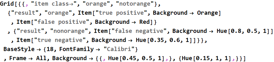
Out[45]=
| item class→ | orange | notorange | |
| result | orange | true positive | false positive |
| result | nonorange | false negative | true negative |
What will happen if we do not teach the classifier well what “notorange” are? Will it be more gullible and think everything is orange (more false positive)? Below is exactly the same thing, but we use a smaller “notorange” set: notorange2
In[59]:=

In[61]:=
![Graphics:PlotLabel /. Options[{RowBox[{RowBox[{data, =, RowBox[{{, RowBox[{GraphicsBox[TagBox[RasterBox[NumericArray[<100,105,3>, UnsignedInteger8], {{0, 100}, {105, 0}}, {0, 255}, ColorFunction -> RGBColor], BoxForm`ImageTag[System`Convert`CommonDump`ConvertText[Byte, System`Convert`HTMLDump`htmlsave, HTMLEntities -> {HTMLBasic}, AltMathOutput -> PlotLabel, WindowSize -> {2000, Automatic}, MathOutput -> PNG, ConvertClosed -> False, ConvertReverseClosed -> False, ConvertLinkedNotebooks -> False, CharacterEncoding -> Automatic, ConversionStyleEnvironment -> None, ConversionRules -> Automatic, HeadAttributes -> {}, HeadElements -> {}, CSS -> Automatic, ConvertLinkedNotebooks -> False, MathOutput -> GIF, GraphicsOutput -> GIF, Graphics3DOutput -> Automatic, ManipulateOutput -> CDF, ConvertClosed -> True, ConvertReverseClosed -> False, FullDocument -> True, AltMathOutput -> FileName, TableOutput -> {TextForm, Automatic}, AnimationOutput -> Automatic, FilesDirectory -> HTMLFiles, LinksDirectory -> HTMLLinks, HTMLEntities -> {HTML}, AllowBlockMathML -> False, ShowStyles -> True, DataUri -> False, MathMLOptions -> {UseUnicodePlane1Characters -> False, IncludeMarkupAnnotations -> False, Entities -> MathML}], ColorSpace -> System`Convert`CommonDump`ConvertText[RGB, System`Convert`HTMLDump`htmlsave, HTMLEntities -> {HTMLBasic}, AltMathOutput -> PlotLabel, WindowSize -> {2000, Automatic}, MathOutput -> PNG, ConvertClosed -> False, ConvertReverseClosed -> False, ConvertLinkedNotebooks -> False, CharacterEncoding -> Automatic, ConversionStyleEnvironment -> None, ConversionRules -> Automatic, HeadAttributes -> {}, HeadElements -> {}, CSS -> Automatic, ConvertLinkedNotebooks -> False, MathOutput -> GIF, GraphicsOutput -> GIF, Graphics3DOutput -> Automatic, ManipulateOutput -> CDF, ConvertClosed -> True, ConvertReverseClosed -> False, FullDocument -> True, AltMathOutput -> FileName, TableOutput -> {TextForm, Automatic}, AnimationOutput -> Automatic, FilesDirectory -> HTMLFiles, LinksDirectory -> HTMLLinks, HTMLEntities -> {HTML}, AllowBlockMathML -> False, ShowStyles -> True, DataUri -> False, MathMLOptions -> {UseUnicodePlane1Characters -> False, IncludeMarkupAnnotations -> False, Entities -> MathML}], Interleaving -> True], Selectable -> False], DefaultBaseStyle -> System`Convert`CommonDump`ConvertText[ImageGraphics, System`Convert`HTMLDump`htmlsave, HTMLEntities -> {HTMLBasic}, AltMathOutput -> PlotLabel, WindowSize -> {2000, Automatic}, MathOutput -> PNG, ConvertClosed -> False, ConvertReverseClosed -> False, ConvertLinkedNotebooks -> False, CharacterEncoding -> Automatic, ConversionStyleEnvironment -> None, ConversionRules -> Automatic, HeadAttributes -> {}, HeadElements -> {}, CSS -> Automatic, ConvertLinkedNotebooks -> False, MathOutput -> GIF, GraphicsOutput -> GIF, Graphics3DOutput -> Automatic, ManipulateOutput -> CDF, ConvertClosed -> True, ConvertReverseClosed -> False, FullDocument -> True, AltMathOutput -> FileName, TableOutput -> {TextForm, Automatic}, AnimationOutput -> Automatic, FilesDirectory -> HTMLFiles, LinksDirectory -> HTMLLinks, HTMLEntities -> {HTML}, AllowBlockMathML -> False, ShowStyles -> True, DataUri -> False, MathMLOptions -> {UseUnicodePlane1Characters -> False, IncludeMarkupAnnotations -> False, Entities -> MathML}], ImageSize -> Automatic, ImageSizeRaw -> {105, 100}, PlotRange -> {{0, 105}, {0, 100}}], ,, GraphicsBox[TagBox[RasterBox[NumericArray[<98,99,3>, UnsignedInteger8], {{0, 98}, {99, 0}}, {0, 255}, ColorFunction -> RGBColor], BoxForm`ImageTag[System`Convert`CommonDump`ConvertText[Byte, System`Convert`HTMLDump`htmlsave, HTMLEntities -> {HTMLBasic}, AltMathOutput -> PlotLabel, WindowSize -> {2000, Automatic}, MathOutput -> PNG, ConvertClosed -> False, ConvertReverseClosed -> False, ConvertLinkedNotebooks -> False, CharacterEncoding -> Automatic, ConversionStyleEnvironment -> None, ConversionRules -> Automatic, HeadAttributes -> {}, HeadElements -> {}, CSS -> Automatic, ConvertLinkedNotebooks -> False, MathOutput -> GIF, GraphicsOutput -> GIF, Graphics3DOutput -> Automatic, ManipulateOutput -> CDF, ConvertClosed -> True, ConvertReverseClosed -> False, FullDocument -> True, AltMathOutput -> FileName, TableOutput -> {TextForm, Automatic}, AnimationOutput -> Automatic, FilesDirectory -> HTMLFiles, LinksDirectory -> HTMLLinks, HTMLEntities -> {HTML}, AllowBlockMathML -> False, ShowStyles -> True, DataUri -> False, MathMLOptions -> {UseUnicodePlane1Characters -> False, IncludeMarkupAnnotations -> False, Entities -> MathML}], ColorSpace -> System`Convert`CommonDump`ConvertText[RGB, System`Convert`HTMLDump`htmlsave, HTMLEntities -> {HTMLBasic}, AltMathOutput -> PlotLabel, WindowSize -> {2000, Automatic}, MathOutput -> PNG, ConvertClosed -> False, ConvertReverseClosed -> False, ConvertLinkedNotebooks -> False, CharacterEncoding -> Automatic, ConversionStyleEnvironment -> None, ConversionRules -> Automatic, HeadAttributes -> {}, HeadElements -> {}, CSS -> Automatic, ConvertLinkedNotebooks -> False, MathOutput -> GIF, GraphicsOutput -> GIF, Graphics3DOutput -> Automatic, ManipulateOutput -> CDF, ConvertClosed -> True, ConvertReverseClosed -> False, FullDocument -> True, AltMathOutput -> FileName, TableOutput -> {TextForm, Automatic}, AnimationOutput -> Automatic, FilesDirectory -> HTMLFiles, LinksDirectory -> HTMLLinks, HTMLEntities -> {HTML}, AllowBlockMathML -> False, ShowStyles -> True, DataUri -> False, MathMLOptions -> {UseUnicodePlane1Characters -> False, IncludeMarkupAnnotations -> False, Entities -> MathML}], Interleaving -> True], Selectable -> False], DefaultBaseStyle -> System`Convert`CommonDump`ConvertText[ImageGraphics, System`Convert`HTMLDump`htmlsave, HTMLEntities -> {HTMLBasic}, AltMathOutput -> PlotLabel, WindowSize -> {2000, Automatic}, MathOutput -> PNG, ConvertClosed -> False, ConvertReverseClosed -> False, ConvertLinkedNotebooks -> False, CharacterEncoding -> Automatic, ConversionStyleEnvironment -> None, ConversionRules -> Automatic, HeadAttributes -> {}, HeadElements -> {}, CSS -> Automatic, ConvertLinkedNotebooks -> False, MathOutput -> GIF, GraphicsOutput -> GIF, Graphics3DOutput -> Automatic, ManipulateOutput -> CDF, ConvertClosed -> True, ConvertReverseClosed -> False, FullDocument -> True, AltMathOutput -> FileName, TableOutput -> {TextForm, Automatic}, AnimationOutput -> Automatic, FilesDirectory -> HTMLFiles, LinksDirectory -> HTMLLinks, HTMLEntities -> {HTML}, AllowBlockMathML -> False, ShowStyles -> True, DataUri -> False, MathMLOptions -> {UseUnicodePlane1Characters -> False, IncludeMarkupAnnotations -> False, Entities -> MathML}], ImageSize -> Automatic, ImageSizeRaw -> {99, 98}, PlotRange -> {{0, 99}, {0, 98}}], ,, GraphicsBox[TagBox[RasterBox[NumericArray[<98,103,3>, UnsignedInteger8], {{0, 98}, {103, 0}}, {0, 255}, ColorFunction -> RGBColor], BoxForm`ImageTag[System`Convert`CommonDump`ConvertText[Byte, System`Convert`HTMLDump`htmlsave, HTMLEntities -> {HTMLBasic}, AltMathOutput -> PlotLabel, WindowSize -> {2000, Automatic}, MathOutput -> PNG, ConvertClosed -> False, ConvertReverseClosed -> False, ConvertLinkedNotebooks -> False, CharacterEncoding -> Automatic, ConversionStyleEnvironment -> None, ConversionRules -> Automatic, HeadAttributes -> {}, HeadElements -> {}, CSS -> Automatic, ConvertLinkedNotebooks -> False, MathOutput -> GIF, GraphicsOutput -> GIF, Graphics3DOutput -> Automatic, ManipulateOutput -> CDF, ConvertClosed -> True, ConvertReverseClosed -> False, FullDocument -> True, AltMathOutput -> FileName, TableOutput -> {TextForm, Automatic}, AnimationOutput -> Automatic, FilesDirectory -> HTMLFiles, LinksDirectory -> HTMLLinks, HTMLEntities -> {HTML}, AllowBlockMathML -> False, ShowStyles -> True, DataUri -> False, MathMLOptions -> {UseUnicodePlane1Characters -> False, IncludeMarkupAnnotations -> False, Entities -> MathML}], ColorSpace -> System`Convert`CommonDump`ConvertText[RGB, System`Convert`HTMLDump`htmlsave, HTMLEntities -> {HTMLBasic}, AltMathOutput -> PlotLabel, WindowSize -> {2000, Automatic}, MathOutput -> PNG, ConvertClosed -> False, ConvertReverseClosed -> False, ConvertLinkedNotebooks -> False, CharacterEncoding -> Automatic, ConversionStyleEnvironment -> None, ConversionRules -> Automatic, HeadAttributes -> {}, HeadElements -> {}, CSS -> Automatic, ConvertLinkedNotebooks -> False, MathOutput -> GIF, GraphicsOutput -> GIF, Graphics3DOutput -> Automatic, ManipulateOutput -> CDF, ConvertClosed -> True, ConvertReverseClosed -> False, FullDocument -> True, AltMathOutput -> FileName, TableOutput -> {TextForm, Automatic}, AnimationOutput -> Automatic, FilesDirectory -> HTMLFiles, LinksDirectory -> HTMLLinks, HTMLEntities -> {HTML}, AllowBlockMathML -> False, ShowStyles -> True, DataUri -> False, MathMLOptions -> {UseUnicodePlane1Characters -> False, IncludeMarkupAnnotations -> False, Entities -> MathML}], Interleaving -> True], Selectable -> False], DefaultBaseStyle -> System`Convert`CommonDump`ConvertText[ImageGraphics, System`Convert`HTMLDump`htmlsave, HTMLEntities -> {HTMLBasic}, AltMathOutput -> PlotLabel, WindowSize -> {2000, Automatic}, MathOutput -> PNG, ConvertClosed -> False, ConvertReverseClosed -> False, ConvertLinkedNotebooks -> False, CharacterEncoding -> Automatic, ConversionStyleEnvironment -> None, ConversionRules -> Automatic, HeadAttributes -> {}, HeadElements -> {}, CSS -> Automatic, ConvertLinkedNotebooks -> False, MathOutput -> GIF, GraphicsOutput -> GIF, Graphics3DOutput -> Automatic, ManipulateOutput -> CDF, ConvertClosed -> True, ConvertReverseClosed -> False, FullDocument -> True, AltMathOutput -> FileName, TableOutput -> {TextForm, Automatic}, AnimationOutput -> Automatic, FilesDirectory -> HTMLFiles, LinksDirectory -> HTMLLinks, HTMLEntities -> {HTML}, AllowBlockMathML -> False, ShowStyles -> True, DataUri -> False, MathMLOptions -> {UseUnicodePlane1Characters -> False, IncludeMarkupAnnotations -> False, Entities -> MathML}], ImageSize -> Automatic, ImageSizeRaw -> {103, 98}, PlotRange -> {{0, 103}, {0, 98}}], ,, orangevalid[[RandomInteger[{1, 5}]]], ,, GraphicsBox[TagBox[RasterBox[NumericArray[<98,102,3>, UnsignedInteger8], {{0, 98}, {102, 0}}, {0, 255}, ColorFunction -> RGBColor], BoxForm`ImageTag[System`Convert`CommonDump`ConvertText[Byte, System`Convert`HTMLDump`htmlsave, HTMLEntities -> {HTMLBasic}, AltMathOutput -> PlotLabel, WindowSize -> {2000, Automatic}, MathOutput -> PNG, ConvertClosed -> False, ConvertReverseClosed -> False, ConvertLinkedNotebooks -> False, CharacterEncoding -> Automatic, ConversionStyleEnvironment -> None, ConversionRules -> Automatic, HeadAttributes -> {}, HeadElements -> {}, CSS -> Automatic, ConvertLinkedNotebooks -> False, MathOutput -> GIF, GraphicsOutput -> GIF, Graphics3DOutput -> Automatic, ManipulateOutput -> CDF, ConvertClosed -> True, ConvertReverseClosed -> False, FullDocument -> True, AltMathOutput -> FileName, TableOutput -> {TextForm, Automatic}, AnimationOutput -> Automatic, FilesDirectory -> HTMLFiles, LinksDirectory -> HTMLLinks, HTMLEntities -> {HTML}, AllowBlockMathML -> False, ShowStyles -> True, DataUri -> False, MathMLOptions -> {UseUnicodePlane1Characters -> False, IncludeMarkupAnnotations -> False, Entities -> MathML}], ColorSpace -> System`Convert`CommonDump`ConvertText[RGB, System`Convert`HTMLDump`htmlsave, HTMLEntities -> {HTMLBasic}, AltMathOutput -> PlotLabel, WindowSize -> {2000, Automatic}, MathOutput -> PNG, ConvertClosed -> False, ConvertReverseClosed -> False, ConvertLinkedNotebooks -> False, CharacterEncoding -> Automatic, ConversionStyleEnvironment -> None, ConversionRules -> Automatic, HeadAttributes -> {}, HeadElements -> {}, CSS -> Automatic, ConvertLinkedNotebooks -> False, MathOutput -> GIF, GraphicsOutput -> GIF, Graphics3DOutput -> Automatic, ManipulateOutput -> CDF, ConvertClosed -> True, ConvertReverseClosed -> False, FullDocument -> True, AltMathOutput -> FileName, TableOutput -> {TextForm, Automatic}, AnimationOutput -> Automatic, FilesDirectory -> HTMLFiles, LinksDirectory -> HTMLLinks, HTMLEntities -> {HTML}, AllowBlockMathML -> False, ShowStyles -> True, DataUri -> False, MathMLOptions -> {UseUnicodePlane1Characters -> False, IncludeMarkupAnnotations -> False, Entities -> MathML}], Interleaving -> True], Selectable -> False], DefaultBaseStyle -> System`Convert`CommonDump`ConvertText[ImageGraphics, System`Convert`HTMLDump`htmlsave, HTMLEntities -> {HTMLBasic}, AltMathOutput -> PlotLabel, WindowSize -> {2000, Automatic}, MathOutput -> PNG, ConvertClosed -> False, ConvertReverseClosed -> False, ConvertLinkedNotebooks -> False, CharacterEncoding -> Automatic, ConversionStyleEnvironment -> None, ConversionRules -> Automatic, HeadAttributes -> {}, HeadElements -> {}, CSS -> Automatic, ConvertLinkedNotebooks -> False, MathOutput -> GIF, GraphicsOutput -> GIF, Graphics3DOutput -> Automatic, ManipulateOutput -> CDF, ConvertClosed -> True, ConvertReverseClosed -> False, FullDocument -> True, AltMathOutput -> FileName, TableOutput -> {TextForm, Automatic}, AnimationOutput -> Automatic, FilesDirectory -> HTMLFiles, LinksDirectory -> HTMLLinks, HTMLEntities -> {HTML}, AllowBlockMathML -> False, ShowStyles -> True, DataUri -> False, MathMLOptions -> {UseUnicodePlane1Characters -> False, IncludeMarkupAnnotations -> False, Entities -> MathML}], ImageSize -> Automatic, ImageSizeRaw -> {102, 98}, PlotRange -> {{0, 102}, {0, 98}}], ,, GraphicsBox[TagBox[RasterBox[NumericArray[<98,101,3>, UnsignedInteger8], {{0, 98}, {101, 0}}, {0, 255}, ColorFunction -> RGBColor], BoxForm`ImageTag[System`Convert`CommonDump`ConvertText[Byte, System`Convert`HTMLDump`htmlsave, HTMLEntities -> {HTMLBasic}, AltMathOutput -> PlotLabel, WindowSize -> {2000, Automatic}, MathOutput -> PNG, ConvertClosed -> False, ConvertReverseClosed -> False, ConvertLinkedNotebooks -> False, CharacterEncoding -> Automatic, ConversionStyleEnvironment -> None, ConversionRules -> Automatic, HeadAttributes -> {}, HeadElements -> {}, CSS -> Automatic, ConvertLinkedNotebooks -> False, MathOutput -> GIF, GraphicsOutput -> GIF, Graphics3DOutput -> Automatic, ManipulateOutput -> CDF, ConvertClosed -> True, ConvertReverseClosed -> False, FullDocument -> True, AltMathOutput -> FileName, TableOutput -> {TextForm, Automatic}, AnimationOutput -> Automatic, FilesDirectory -> HTMLFiles, LinksDirectory -> HTMLLinks, HTMLEntities -> {HTML}, AllowBlockMathML -> False, ShowStyles -> True, DataUri -> False, MathMLOptions -> {UseUnicodePlane1Characters -> False, IncludeMarkupAnnotations -> False, Entities -> MathML}], ColorSpace -> System`Convert`CommonDump`ConvertText[RGB, System`Convert`HTMLDump`htmlsave, HTMLEntities -> {HTMLBasic}, AltMathOutput -> PlotLabel, WindowSize -> {2000, Automatic}, MathOutput -> PNG, ConvertClosed -> False, ConvertReverseClosed -> False, ConvertLinkedNotebooks -> False, CharacterEncoding -> Automatic, ConversionStyleEnvironment -> None, ConversionRules -> Automatic, HeadAttributes -> {}, HeadElements -> {}, CSS -> Automatic, ConvertLinkedNotebooks -> False, MathOutput -> GIF, GraphicsOutput -> GIF, Graphics3DOutput -> Automatic, ManipulateOutput -> CDF, ConvertClosed -> True, ConvertReverseClosed -> False, FullDocument -> True, AltMathOutput -> FileName, TableOutput -> {TextForm, Automatic}, AnimationOutput -> Automatic, FilesDirectory -> HTMLFiles, LinksDirectory -> HTMLLinks, HTMLEntities -> {HTML}, AllowBlockMathML -> False, ShowStyles -> True, DataUri -> False, MathMLOptions -> {UseUnicodePlane1Characters -> False, IncludeMarkupAnnotations -> False, Entities -> MathML}], Interleaving -> True], Selectable -> False], DefaultBaseStyle -> System`Convert`CommonDump`ConvertText[ImageGraphics, System`Convert`HTMLDump`htmlsave, HTMLEntities -> {HTMLBasic}, AltMathOutput -> PlotLabel, WindowSize -> {2000, Automatic}, MathOutput -> PNG, ConvertClosed -> False, ConvertReverseClosed -> False, ConvertLinkedNotebooks -> False, CharacterEncoding -> Automatic, ConversionStyleEnvironment -> None, ConversionRules -> Automatic, HeadAttributes -> {}, HeadElements -> {}, CSS -> Automatic, ConvertLinkedNotebooks -> False, MathOutput -> GIF, GraphicsOutput -> GIF, Graphics3DOutput -> Automatic, ManipulateOutput -> CDF, ConvertClosed -> True, ConvertReverseClosed -> False, FullDocument -> True, AltMathOutput -> FileName, TableOutput -> {TextForm, Automatic}, AnimationOutput -> Automatic, FilesDirectory -> HTMLFiles, LinksDirectory -> HTMLLinks, HTMLEntities -> {HTML}, AllowBlockMathML -> False, ShowStyles -> True, DataUri -> False, MathMLOptions -> {UseUnicodePlane1Characters -> False, IncludeMarkupAnnotations -> False, Entities -> MathML}], ImageSize -> Automatic, ImageSizeRaw -> {101, 98}, PlotRange -> {{0, 101}, {0, 98}}], ,, GraphicsBox[TagBox[RasterBox[NumericArray[<97,99,3>, UnsignedInteger8], {{0, 97}, {99, 0}}, {0, 255}, ColorFunction -> RGBColor], BoxForm`ImageTag[System`Convert`CommonDump`ConvertText[Byte, System`Convert`HTMLDump`htmlsave, HTMLEntities -> {HTMLBasic}, AltMathOutput -> PlotLabel, WindowSize -> {2000, Automatic}, MathOutput -> PNG, ConvertClosed -> False, ConvertReverseClosed -> False, ConvertLinkedNotebooks -> False, CharacterEncoding -> Automatic, ConversionStyleEnvironment -> None, ConversionRules -> Automatic, HeadAttributes -> {}, HeadElements -> {}, CSS -> Automatic, ConvertLinkedNotebooks -> False, MathOutput -> GIF, GraphicsOutput -> GIF, Graphics3DOutput -> Automatic, ManipulateOutput -> CDF, ConvertClosed -> True, ConvertReverseClosed -> False, FullDocument -> True, AltMathOutput -> FileName, TableOutput -> {TextForm, Automatic}, AnimationOutput -> Automatic, FilesDirectory -> HTMLFiles, LinksDirectory -> HTMLLinks, HTMLEntities -> {HTML}, AllowBlockMathML -> False, ShowStyles -> True, DataUri -> False, MathMLOptions -> {UseUnicodePlane1Characters -> False, IncludeMarkupAnnotations -> False, Entities -> MathML}], ColorSpace -> System`Convert`CommonDump`ConvertText[RGB, System`Convert`HTMLDump`htmlsave, HTMLEntities -> {HTMLBasic}, AltMathOutput -> PlotLabel, WindowSize -> {2000, Automatic}, MathOutput -> PNG, ConvertClosed -> False, ConvertReverseClosed -> False, ConvertLinkedNotebooks -> False, CharacterEncoding -> Automatic, ConversionStyleEnvironment -> None, ConversionRules -> Automatic, HeadAttributes -> {}, HeadElements -> {}, CSS -> Automatic, ConvertLinkedNotebooks -> False, MathOutput -> GIF, GraphicsOutput -> GIF, Graphics3DOutput -> Automatic, ManipulateOutput -> CDF, ConvertClosed -> True, ConvertReverseClosed -> False, FullDocument -> True, AltMathOutput -> FileName, TableOutput -> {TextForm, Automatic}, AnimationOutput -> Automatic, FilesDirectory -> HTMLFiles, LinksDirectory -> HTMLLinks, HTMLEntities -> {HTML}, AllowBlockMathML -> False, ShowStyles -> True, DataUri -> False, MathMLOptions -> {UseUnicodePlane1Characters -> False, IncludeMarkupAnnotations -> False, Entities -> MathML}], Interleaving -> True], Selectable -> False], DefaultBaseStyle -> System`Convert`CommonDump`ConvertText[ImageGraphics, System`Convert`HTMLDump`htmlsave, HTMLEntities -> {HTMLBasic}, AltMathOutput -> PlotLabel, WindowSize -> {2000, Automatic}, MathOutput -> PNG, ConvertClosed -> False, ConvertReverseClosed -> False, ConvertLinkedNotebooks -> False, CharacterEncoding -> Automatic, ConversionStyleEnvironment -> None, ConversionRules -> Automatic, HeadAttributes -> {}, HeadElements -> {}, CSS -> Automatic, ConvertLinkedNotebooks -> False, MathOutput -> GIF, GraphicsOutput -> GIF, Graphics3DOutput -> Automatic, ManipulateOutput -> CDF, ConvertClosed -> True, ConvertReverseClosed -> False, FullDocument -> True, AltMathOutput -> FileName, TableOutput -> {TextForm, Automatic}, AnimationOutput -> Automatic, FilesDirectory -> HTMLFiles, LinksDirectory -> HTMLLinks, HTMLEntities -> {HTML}, AllowBlockMathML -> False, ShowStyles -> True, DataUri -> False, MathMLOptions -> {UseUnicodePlane1Characters -> False, IncludeMarkupAnnotations -> False, Entities -> MathML}], ImageSize -> Automatic, ImageSizeRaw -> {99, 97}, PlotRange -> {{0, 99}, {0, 97}}], ,, GraphicsBox[TagBox[RasterBox[NumericArray[<93,96,3>, UnsignedInteger8], {{0, 93}, {96, 0}}, {0, 255}, ColorFunction -> RGBColor], BoxForm`ImageTag[System`Convert`CommonDump`ConvertText[Byte, System`Convert`HTMLDump`htmlsave, HTMLEntities -> {HTMLBasic}, AltMathOutput -> PlotLabel, WindowSize -> {2000, Automatic}, MathOutput -> PNG, ConvertClosed -> False, ConvertReverseClosed -> False, ConvertLinkedNotebooks -> False, CharacterEncoding -> Automatic, ConversionStyleEnvironment -> None, ConversionRules -> Automatic, HeadAttributes -> {}, HeadElements -> {}, CSS -> Automatic, ConvertLinkedNotebooks -> False, MathOutput -> GIF, GraphicsOutput -> GIF, Graphics3DOutput -> Automatic, ManipulateOutput -> CDF, ConvertClosed -> True, ConvertReverseClosed -> False, FullDocument -> True, AltMathOutput -> FileName, TableOutput -> {TextForm, Automatic}, AnimationOutput -> Automatic, FilesDirectory -> HTMLFiles, LinksDirectory -> HTMLLinks, HTMLEntities -> {HTML}, AllowBlockMathML -> False, ShowStyles -> True, DataUri -> False, MathMLOptions -> {UseUnicodePlane1Characters -> False, IncludeMarkupAnnotations -> False, Entities -> MathML}], ColorSpace -> System`Convert`CommonDump`ConvertText[RGB, System`Convert`HTMLDump`htmlsave, HTMLEntities -> {HTMLBasic}, AltMathOutput -> PlotLabel, WindowSize -> {2000, Automatic}, MathOutput -> PNG, ConvertClosed -> False, ConvertReverseClosed -> False, ConvertLinkedNotebooks -> False, CharacterEncoding -> Automatic, ConversionStyleEnvironment -> None, ConversionRules -> Automatic, HeadAttributes -> {}, HeadElements -> {}, CSS -> Automatic, ConvertLinkedNotebooks -> False, MathOutput -> GIF, GraphicsOutput -> GIF, Graphics3DOutput -> Automatic, ManipulateOutput -> CDF, ConvertClosed -> True, ConvertReverseClosed -> False, FullDocument -> True, AltMathOutput -> FileName, TableOutput -> {TextForm, Automatic}, AnimationOutput -> Automatic, FilesDirectory -> HTMLFiles, LinksDirectory -> HTMLLinks, HTMLEntities -> {HTML}, AllowBlockMathML -> False, ShowStyles -> True, DataUri -> False, MathMLOptions -> {UseUnicodePlane1Characters -> False, IncludeMarkupAnnotations -> False, Entities -> MathML}], Interleaving -> True], Selectable -> False], DefaultBaseStyle -> System`Convert`CommonDump`ConvertText[ImageGraphics, System`Convert`HTMLDump`htmlsave, HTMLEntities -> {HTMLBasic}, AltMathOutput -> PlotLabel, WindowSize -> {2000, Automatic}, MathOutput -> PNG, ConvertClosed -> False, ConvertReverseClosed -> False, ConvertLinkedNotebooks -> False, CharacterEncoding -> Automatic, ConversionStyleEnvironment -> None, ConversionRules -> Automatic, HeadAttributes -> {}, HeadElements -> {}, CSS -> Automatic, ConvertLinkedNotebooks -> False, MathOutput -> GIF, GraphicsOutput -> GIF, Graphics3DOutput -> Automatic, ManipulateOutput -> CDF, ConvertClosed -> True, ConvertReverseClosed -> False, FullDocument -> True, AltMathOutput -> FileName, TableOutput -> {TextForm, Automatic}, AnimationOutput -> Automatic, FilesDirectory -> HTMLFiles, LinksDirectory -> HTMLLinks, HTMLEntities -> {HTML}, AllowBlockMathML -> False, ShowStyles -> True, DataUri -> False, MathMLOptions -> {UseUnicodePlane1Characters -> False, IncludeMarkupAnnotations -> False, Entities -> MathML}], ImageSize -> Automatic, ImageSizeRaw -> {96, 93}, PlotRange -> {{0, 96}, {0, 93}}], ,, GraphicsBox[TagBox[RasterBox[NumericArray[<99,102,3>, UnsignedInteger8], {{0, 99}, {102, 0}}, {0, 255}, ColorFunction -> RGBColor], BoxForm`ImageTag[System`Convert`CommonDump`ConvertText[Byte, System`Convert`HTMLDump`htmlsave, HTMLEntities -> {HTMLBasic}, AltMathOutput -> PlotLabel, WindowSize -> {2000, Automatic}, MathOutput -> PNG, ConvertClosed -> False, ConvertReverseClosed -> False, ConvertLinkedNotebooks -> False, CharacterEncoding -> Automatic, ConversionStyleEnvironment -> None, ConversionRules -> Automatic, HeadAttributes -> {}, HeadElements -> {}, CSS -> Automatic, ConvertLinkedNotebooks -> False, MathOutput -> GIF, GraphicsOutput -> GIF, Graphics3DOutput -> Automatic, ManipulateOutput -> CDF, ConvertClosed -> True, ConvertReverseClosed -> False, FullDocument -> True, AltMathOutput -> FileName, TableOutput -> {TextForm, Automatic}, AnimationOutput -> Automatic, FilesDirectory -> HTMLFiles, LinksDirectory -> HTMLLinks, HTMLEntities -> {HTML}, AllowBlockMathML -> False, ShowStyles -> True, DataUri -> False, MathMLOptions -> {UseUnicodePlane1Characters -> False, IncludeMarkupAnnotations -> False, Entities -> MathML}], ColorSpace -> System`Convert`CommonDump`ConvertText[RGB, System`Convert`HTMLDump`htmlsave, HTMLEntities -> {HTMLBasic}, AltMathOutput -> PlotLabel, WindowSize -> {2000, Automatic}, MathOutput -> PNG, ConvertClosed -> False, ConvertReverseClosed -> False, ConvertLinkedNotebooks -> False, CharacterEncoding -> Automatic, ConversionStyleEnvironment -> None, ConversionRules -> Automatic, HeadAttributes -> {}, HeadElements -> {}, CSS -> Automatic, ConvertLinkedNotebooks -> False, MathOutput -> GIF, GraphicsOutput -> GIF, Graphics3DOutput -> Automatic, ManipulateOutput -> CDF, ConvertClosed -> True, ConvertReverseClosed -> False, FullDocument -> True, AltMathOutput -> FileName, TableOutput -> {TextForm, Automatic}, AnimationOutput -> Automatic, FilesDirectory -> HTMLFiles, LinksDirectory -> HTMLLinks, HTMLEntities -> {HTML}, AllowBlockMathML -> False, ShowStyles -> True, DataUri -> False, MathMLOptions -> {UseUnicodePlane1Characters -> False, IncludeMarkupAnnotations -> False, Entities -> MathML}], Interleaving -> True], Selectable -> False], DefaultBaseStyle -> System`Convert`CommonDump`ConvertText[ImageGraphics, System`Convert`HTMLDump`htmlsave, HTMLEntities -> {HTMLBasic}, AltMathOutput -> PlotLabel, WindowSize -> {2000, Automatic}, MathOutput -> PNG, ConvertClosed -> False, ConvertReverseClosed -> False, ConvertLinkedNotebooks -> False, CharacterEncoding -> Automatic, ConversionStyleEnvironment -> None, ConversionRules -> Automatic, HeadAttributes -> {}, HeadElements -> {}, CSS -> Automatic, ConvertLinkedNotebooks -> False, MathOutput -> GIF, GraphicsOutput -> GIF, Graphics3DOutput -> Automatic, ManipulateOutput -> CDF, ConvertClosed -> True, ConvertReverseClosed -> False, FullDocument -> True, AltMathOutput -> FileName, TableOutput -> {TextForm, Automatic}, AnimationOutput -> Automatic, FilesDirectory -> HTMLFiles, LinksDirectory -> HTMLLinks, HTMLEntities -> {HTML}, AllowBlockMathML -> False, ShowStyles -> True, DataUri -> False, MathMLOptions -> {UseUnicodePlane1Characters -> False, IncludeMarkupAnnotations -> False, Entities -> MathML}], ImageSize -> Automatic, ImageSizeRaw -> {102, 99}, PlotRange -> {{0, 102}, {0, 99}}]}], }}]}], ;}], , Grid[MapThread[Prepend, {Join[{data}, Table[Table[res = c[data[[j]]] ; Item[res, Background→If[TrueQ[res == orange], If[ MemberQ[{1, 4, 9}, j], Orange, Red] , If[ MemberQ[{1, 4, 9}, j], Hue[0.8, 0.5, 1], Hue[0.35, 0.6, 1]]]], {j, 1, Length @ data}] , {c, classOr2}]] , Join[{}, StringTake[#, Min[14, StringLength[#]]] & /@ method]}], BaseStyle→ {16}]}]](HTMLFiles/LectNotes_intro_data_analytics_260.gif)
Out[62]=
 |
 |
 |
 |
 |
 |
 |
 |
 |
|
| SupportVectorM | orange | notorange | notorange | orange | notorange | notorange | notorange | notorange | orange |
| NaiveBayes | orange | orange | notorange | orange | notorange | notorange | notorange | notorange | orange |
| LogisticRegres | orange | orange | orange | orange | orange | notorange | notorange | notorange | orange |
| NeuralNetwork | orange | orange | orange | orange | orange | orange | orange | orange | orange |
| NearestNeighbo | orange | orange | orange | orange | orange | orange | orange | notorange | orange |
| RandomForest | orange | notorange | notorange | orange | notorange | notorange | notorange | notorange | orange |
| Markov2 | notorange | notorange | notorange | orange | notorange | notorange | notorange | notorange | notorange |
| PriorBaseline | orange | orange | orange | orange | orange | orange | orange | orange | orange |
| UniformBaselin | orange | orange | orange | orange | orange | orange | orange | orange | orange |
Indeed, there are a lot more red: false positive. But also more orange: true positive. The trade-off between false positive - true positive can be plot as a curve called “Receiver Operation Characteristics” or ROC back from WW2 radar development days.
Why does the calculation take so long? This is why:

![]()
The classifiers have to go through 53 M numbers. That is the reason why it is not practical for a small PC to run big classification job - not sufficient memory and it will take forever. What we see in the above, such as:  is really the tip of the iceberg, as the model crunches through the huge number of data and stores the model parameters within itself to do any computing when it is called.
Big real world classifiers, speech, image recognition are done by big cloud computing.
As a side note. you might have seen the below, it is about classification with method “RandomForest”

Their training set is ~500,000 songs! imagine the number crunching through that, and random forest is particularly suited to categorical classification like this. How good is the classification?
That kind of number is already quite good for complex social phenomena like this.
5. Classify exercise : beverage images
In[44]:=
![Graphics:PlotLabel /. Options[{RowBox[{RowBox[{coffee, =, RowBox[{{, RowBox[{GraphicsBox[TagBox[RasterBox[NumericArray[<113,150,4>, UnsignedInteger8], {{0, 113}, {150, 0}}, {0, 255}, ColorFunction -> RGBColor], BoxForm`ImageTag[System`Convert`CommonDump`ConvertText[Byte, System`Convert`HTMLDump`htmlsave, HTMLEntities -> {HTMLBasic}, AltMathOutput -> PlotLabel, WindowSize -> {2000, Automatic}, MathOutput -> PNG, ConvertClosed -> False, ConvertReverseClosed -> False, ConvertLinkedNotebooks -> False, CharacterEncoding -> Automatic, ConversionStyleEnvironment -> None, ConversionRules -> Automatic, HeadAttributes -> {}, HeadElements -> {}, CSS -> Automatic, ConvertLinkedNotebooks -> False, MathOutput -> GIF, GraphicsOutput -> GIF, Graphics3DOutput -> Automatic, ManipulateOutput -> CDF, ConvertClosed -> True, ConvertReverseClosed -> False, FullDocument -> True, AltMathOutput -> FileName, TableOutput -> {TextForm, Automatic}, AnimationOutput -> Automatic, FilesDirectory -> HTMLFiles, LinksDirectory -> HTMLLinks, HTMLEntities -> {HTML}, AllowBlockMathML -> False, ShowStyles -> True, DataUri -> False, MathMLOptions -> {UseUnicodePlane1Characters -> False, IncludeMarkupAnnotations -> False, Entities -> MathML}], ColorSpace -> System`Convert`CommonDump`ConvertText[RGB, System`Convert`HTMLDump`htmlsave, HTMLEntities -> {HTMLBasic}, AltMathOutput -> PlotLabel, WindowSize -> {2000, Automatic}, MathOutput -> PNG, ConvertClosed -> False, ConvertReverseClosed -> False, ConvertLinkedNotebooks -> False, CharacterEncoding -> Automatic, ConversionStyleEnvironment -> None, ConversionRules -> Automatic, HeadAttributes -> {}, HeadElements -> {}, CSS -> Automatic, ConvertLinkedNotebooks -> False, MathOutput -> GIF, GraphicsOutput -> GIF, Graphics3DOutput -> Automatic, ManipulateOutput -> CDF, ConvertClosed -> True, ConvertReverseClosed -> False, FullDocument -> True, AltMathOutput -> FileName, TableOutput -> {TextForm, Automatic}, AnimationOutput -> Automatic, FilesDirectory -> HTMLFiles, LinksDirectory -> HTMLLinks, HTMLEntities -> {HTML}, AllowBlockMathML -> False, ShowStyles -> True, DataUri -> False, MathMLOptions -> {UseUnicodePlane1Characters -> False, IncludeMarkupAnnotations -> False, Entities -> MathML}], Interleaving -> True], Selectable -> False], DefaultBaseStyle -> System`Convert`CommonDump`ConvertText[ImageGraphics, System`Convert`HTMLDump`htmlsave, HTMLEntities -> {HTMLBasic}, AltMathOutput -> PlotLabel, WindowSize -> {2000, Automatic}, MathOutput -> PNG, ConvertClosed -> False, ConvertReverseClosed -> False, ConvertLinkedNotebooks -> False, CharacterEncoding -> Automatic, ConversionStyleEnvironment -> None, ConversionRules -> Automatic, HeadAttributes -> {}, HeadElements -> {}, CSS -> Automatic, ConvertLinkedNotebooks -> False, MathOutput -> GIF, GraphicsOutput -> GIF, Graphics3DOutput -> Automatic, ManipulateOutput -> CDF, ConvertClosed -> True, ConvertReverseClosed -> False, FullDocument -> True, AltMathOutput -> FileName, TableOutput -> {TextForm, Automatic}, AnimationOutput -> Automatic, FilesDirectory -> HTMLFiles, LinksDirectory -> HTMLLinks, HTMLEntities -> {HTML}, AllowBlockMathML -> False, ShowStyles -> True, DataUri -> False, MathMLOptions -> {UseUnicodePlane1Characters -> False, IncludeMarkupAnnotations -> False, Entities -> MathML}], ImageSizeRaw -> {150, 113}, PlotRange -> {{0, 150}, {0, 113}}], ,, GraphicsBox[TagBox[RasterBox[NumericArray[<94,150,4>, UnsignedInteger8], {{0, 94}, {150, 0}}, {0, 255}, ColorFunction -> RGBColor], BoxForm`ImageTag[System`Convert`CommonDump`ConvertText[Byte, System`Convert`HTMLDump`htmlsave, HTMLEntities -> {HTMLBasic}, AltMathOutput -> PlotLabel, WindowSize -> {2000, Automatic}, MathOutput -> PNG, ConvertClosed -> False, ConvertReverseClosed -> False, ConvertLinkedNotebooks -> False, CharacterEncoding -> Automatic, ConversionStyleEnvironment -> None, ConversionRules -> Automatic, HeadAttributes -> {}, HeadElements -> {}, CSS -> Automatic, ConvertLinkedNotebooks -> False, MathOutput -> GIF, GraphicsOutput -> GIF, Graphics3DOutput -> Automatic, ManipulateOutput -> CDF, ConvertClosed -> True, ConvertReverseClosed -> False, FullDocument -> True, AltMathOutput -> FileName, TableOutput -> {TextForm, Automatic}, AnimationOutput -> Automatic, FilesDirectory -> HTMLFiles, LinksDirectory -> HTMLLinks, HTMLEntities -> {HTML}, AllowBlockMathML -> False, ShowStyles -> True, DataUri -> False, MathMLOptions -> {UseUnicodePlane1Characters -> False, IncludeMarkupAnnotations -> False, Entities -> MathML}], ColorSpace -> System`Convert`CommonDump`ConvertText[RGB, System`Convert`HTMLDump`htmlsave, HTMLEntities -> {HTMLBasic}, AltMathOutput -> PlotLabel, WindowSize -> {2000, Automatic}, MathOutput -> PNG, ConvertClosed -> False, ConvertReverseClosed -> False, ConvertLinkedNotebooks -> False, CharacterEncoding -> Automatic, ConversionStyleEnvironment -> None, ConversionRules -> Automatic, HeadAttributes -> {}, HeadElements -> {}, CSS -> Automatic, ConvertLinkedNotebooks -> False, MathOutput -> GIF, GraphicsOutput -> GIF, Graphics3DOutput -> Automatic, ManipulateOutput -> CDF, ConvertClosed -> True, ConvertReverseClosed -> False, FullDocument -> True, AltMathOutput -> FileName, TableOutput -> {TextForm, Automatic}, AnimationOutput -> Automatic, FilesDirectory -> HTMLFiles, LinksDirectory -> HTMLLinks, HTMLEntities -> {HTML}, AllowBlockMathML -> False, ShowStyles -> True, DataUri -> False, MathMLOptions -> {UseUnicodePlane1Characters -> False, IncludeMarkupAnnotations -> False, Entities -> MathML}], Interleaving -> True], Selectable -> False], DefaultBaseStyle -> System`Convert`CommonDump`ConvertText[ImageGraphics, System`Convert`HTMLDump`htmlsave, HTMLEntities -> {HTMLBasic}, AltMathOutput -> PlotLabel, WindowSize -> {2000, Automatic}, MathOutput -> PNG, ConvertClosed -> False, ConvertReverseClosed -> False, ConvertLinkedNotebooks -> False, CharacterEncoding -> Automatic, ConversionStyleEnvironment -> None, ConversionRules -> Automatic, HeadAttributes -> {}, HeadElements -> {}, CSS -> Automatic, ConvertLinkedNotebooks -> False, MathOutput -> GIF, GraphicsOutput -> GIF, Graphics3DOutput -> Automatic, ManipulateOutput -> CDF, ConvertClosed -> True, ConvertReverseClosed -> False, FullDocument -> True, AltMathOutput -> FileName, TableOutput -> {TextForm, Automatic}, AnimationOutput -> Automatic, FilesDirectory -> HTMLFiles, LinksDirectory -> HTMLLinks, HTMLEntities -> {HTML}, AllowBlockMathML -> False, ShowStyles -> True, DataUri -> False, MathMLOptions -> {UseUnicodePlane1Characters -> False, IncludeMarkupAnnotations -> False, Entities -> MathML}], ImageSizeRaw -> {150, 94}, PlotRange -> {{0, 150}, {0, 94}}], ,, GraphicsBox[TagBox[RasterBox[NumericArray[<100,150,4>, UnsignedInteger8], {{0, 100}, {150, 0}}, {0, 255}, ColorFunction -> RGBColor], BoxForm`ImageTag[System`Convert`CommonDump`ConvertText[Byte, System`Convert`HTMLDump`htmlsave, HTMLEntities -> {HTMLBasic}, AltMathOutput -> PlotLabel, WindowSize -> {2000, Automatic}, MathOutput -> PNG, ConvertClosed -> False, ConvertReverseClosed -> False, ConvertLinkedNotebooks -> False, CharacterEncoding -> Automatic, ConversionStyleEnvironment -> None, ConversionRules -> Automatic, HeadAttributes -> {}, HeadElements -> {}, CSS -> Automatic, ConvertLinkedNotebooks -> False, MathOutput -> GIF, GraphicsOutput -> GIF, Graphics3DOutput -> Automatic, ManipulateOutput -> CDF, ConvertClosed -> True, ConvertReverseClosed -> False, FullDocument -> True, AltMathOutput -> FileName, TableOutput -> {TextForm, Automatic}, AnimationOutput -> Automatic, FilesDirectory -> HTMLFiles, LinksDirectory -> HTMLLinks, HTMLEntities -> {HTML}, AllowBlockMathML -> False, ShowStyles -> True, DataUri -> False, MathMLOptions -> {UseUnicodePlane1Characters -> False, IncludeMarkupAnnotations -> False, Entities -> MathML}], ColorSpace -> System`Convert`CommonDump`ConvertText[RGB, System`Convert`HTMLDump`htmlsave, HTMLEntities -> {HTMLBasic}, AltMathOutput -> PlotLabel, WindowSize -> {2000, Automatic}, MathOutput -> PNG, ConvertClosed -> False, ConvertReverseClosed -> False, ConvertLinkedNotebooks -> False, CharacterEncoding -> Automatic, ConversionStyleEnvironment -> None, ConversionRules -> Automatic, HeadAttributes -> {}, HeadElements -> {}, CSS -> Automatic, ConvertLinkedNotebooks -> False, MathOutput -> GIF, GraphicsOutput -> GIF, Graphics3DOutput -> Automatic, ManipulateOutput -> CDF, ConvertClosed -> True, ConvertReverseClosed -> False, FullDocument -> True, AltMathOutput -> FileName, TableOutput -> {TextForm, Automatic}, AnimationOutput -> Automatic, FilesDirectory -> HTMLFiles, LinksDirectory -> HTMLLinks, HTMLEntities -> {HTML}, AllowBlockMathML -> False, ShowStyles -> True, DataUri -> False, MathMLOptions -> {UseUnicodePlane1Characters -> False, IncludeMarkupAnnotations -> False, Entities -> MathML}], Interleaving -> True], Selectable -> False], DefaultBaseStyle -> System`Convert`CommonDump`ConvertText[ImageGraphics, System`Convert`HTMLDump`htmlsave, HTMLEntities -> {HTMLBasic}, AltMathOutput -> PlotLabel, WindowSize -> {2000, Automatic}, MathOutput -> PNG, ConvertClosed -> False, ConvertReverseClosed -> False, ConvertLinkedNotebooks -> False, CharacterEncoding -> Automatic, ConversionStyleEnvironment -> None, ConversionRules -> Automatic, HeadAttributes -> {}, HeadElements -> {}, CSS -> Automatic, ConvertLinkedNotebooks -> False, MathOutput -> GIF, GraphicsOutput -> GIF, Graphics3DOutput -> Automatic, ManipulateOutput -> CDF, ConvertClosed -> True, ConvertReverseClosed -> False, FullDocument -> True, AltMathOutput -> FileName, TableOutput -> {TextForm, Automatic}, AnimationOutput -> Automatic, FilesDirectory -> HTMLFiles, LinksDirectory -> HTMLLinks, HTMLEntities -> {HTML}, AllowBlockMathML -> False, ShowStyles -> True, DataUri -> False, MathMLOptions -> {UseUnicodePlane1Characters -> False, IncludeMarkupAnnotations -> False, Entities -> MathML}], ImageSizeRaw -> {150, 100}, PlotRange -> {{0, 150}, {0, 100}}], ,, GraphicsBox[TagBox[RasterBox[NumericArray[<100,150,4>, UnsignedInteger8], {{0, 100}, {150, 0}}, {0, 255}, ColorFunction -> RGBColor], BoxForm`ImageTag[System`Convert`CommonDump`ConvertText[Byte, System`Convert`HTMLDump`htmlsave, HTMLEntities -> {HTMLBasic}, AltMathOutput -> PlotLabel, WindowSize -> {2000, Automatic}, MathOutput -> PNG, ConvertClosed -> False, ConvertReverseClosed -> False, ConvertLinkedNotebooks -> False, CharacterEncoding -> Automatic, ConversionStyleEnvironment -> None, ConversionRules -> Automatic, HeadAttributes -> {}, HeadElements -> {}, CSS -> Automatic, ConvertLinkedNotebooks -> False, MathOutput -> GIF, GraphicsOutput -> GIF, Graphics3DOutput -> Automatic, ManipulateOutput -> CDF, ConvertClosed -> True, ConvertReverseClosed -> False, FullDocument -> True, AltMathOutput -> FileName, TableOutput -> {TextForm, Automatic}, AnimationOutput -> Automatic, FilesDirectory -> HTMLFiles, LinksDirectory -> HTMLLinks, HTMLEntities -> {HTML}, AllowBlockMathML -> False, ShowStyles -> True, DataUri -> False, MathMLOptions -> {UseUnicodePlane1Characters -> False, IncludeMarkupAnnotations -> False, Entities -> MathML}], ColorSpace -> System`Convert`CommonDump`ConvertText[RGB, System`Convert`HTMLDump`htmlsave, HTMLEntities -> {HTMLBasic}, AltMathOutput -> PlotLabel, WindowSize -> {2000, Automatic}, MathOutput -> PNG, ConvertClosed -> False, ConvertReverseClosed -> False, ConvertLinkedNotebooks -> False, CharacterEncoding -> Automatic, ConversionStyleEnvironment -> None, ConversionRules -> Automatic, HeadAttributes -> {}, HeadElements -> {}, CSS -> Automatic, ConvertLinkedNotebooks -> False, MathOutput -> GIF, GraphicsOutput -> GIF, Graphics3DOutput -> Automatic, ManipulateOutput -> CDF, ConvertClosed -> True, ConvertReverseClosed -> False, FullDocument -> True, AltMathOutput -> FileName, TableOutput -> {TextForm, Automatic}, AnimationOutput -> Automatic, FilesDirectory -> HTMLFiles, LinksDirectory -> HTMLLinks, HTMLEntities -> {HTML}, AllowBlockMathML -> False, ShowStyles -> True, DataUri -> False, MathMLOptions -> {UseUnicodePlane1Characters -> False, IncludeMarkupAnnotations -> False, Entities -> MathML}], Interleaving -> True], Selectable -> False], DefaultBaseStyle -> System`Convert`CommonDump`ConvertText[ImageGraphics, System`Convert`HTMLDump`htmlsave, HTMLEntities -> {HTMLBasic}, AltMathOutput -> PlotLabel, WindowSize -> {2000, Automatic}, MathOutput -> PNG, ConvertClosed -> False, ConvertReverseClosed -> False, ConvertLinkedNotebooks -> False, CharacterEncoding -> Automatic, ConversionStyleEnvironment -> None, ConversionRules -> Automatic, HeadAttributes -> {}, HeadElements -> {}, CSS -> Automatic, ConvertLinkedNotebooks -> False, MathOutput -> GIF, GraphicsOutput -> GIF, Graphics3DOutput -> Automatic, ManipulateOutput -> CDF, ConvertClosed -> True, ConvertReverseClosed -> False, FullDocument -> True, AltMathOutput -> FileName, TableOutput -> {TextForm, Automatic}, AnimationOutput -> Automatic, FilesDirectory -> HTMLFiles, LinksDirectory -> HTMLLinks, HTMLEntities -> {HTML}, AllowBlockMathML -> False, ShowStyles -> True, DataUri -> False, MathMLOptions -> {UseUnicodePlane1Characters -> False, IncludeMarkupAnnotations -> False, Entities -> MathML}], ImageSizeRaw -> {150, 100}, PlotRange -> {{0, 150}, {0, 100}}], ,, GraphicsBox[TagBox[RasterBox[NumericArray[<100,150,4>, UnsignedInteger8], {{0, 100}, {150, 0}}, {0, 255}, ColorFunction -> RGBColor], BoxForm`ImageTag[System`Convert`CommonDump`ConvertText[Byte, System`Convert`HTMLDump`htmlsave, HTMLEntities -> {HTMLBasic}, AltMathOutput -> PlotLabel, WindowSize -> {2000, Automatic}, MathOutput -> PNG, ConvertClosed -> False, ConvertReverseClosed -> False, ConvertLinkedNotebooks -> False, CharacterEncoding -> Automatic, ConversionStyleEnvironment -> None, ConversionRules -> Automatic, HeadAttributes -> {}, HeadElements -> {}, CSS -> Automatic, ConvertLinkedNotebooks -> False, MathOutput -> GIF, GraphicsOutput -> GIF, Graphics3DOutput -> Automatic, ManipulateOutput -> CDF, ConvertClosed -> True, ConvertReverseClosed -> False, FullDocument -> True, AltMathOutput -> FileName, TableOutput -> {TextForm, Automatic}, AnimationOutput -> Automatic, FilesDirectory -> HTMLFiles, LinksDirectory -> HTMLLinks, HTMLEntities -> {HTML}, AllowBlockMathML -> False, ShowStyles -> True, DataUri -> False, MathMLOptions -> {UseUnicodePlane1Characters -> False, IncludeMarkupAnnotations -> False, Entities -> MathML}], ColorSpace -> System`Convert`CommonDump`ConvertText[RGB, System`Convert`HTMLDump`htmlsave, HTMLEntities -> {HTMLBasic}, AltMathOutput -> PlotLabel, WindowSize -> {2000, Automatic}, MathOutput -> PNG, ConvertClosed -> False, ConvertReverseClosed -> False, ConvertLinkedNotebooks -> False, CharacterEncoding -> Automatic, ConversionStyleEnvironment -> None, ConversionRules -> Automatic, HeadAttributes -> {}, HeadElements -> {}, CSS -> Automatic, ConvertLinkedNotebooks -> False, MathOutput -> GIF, GraphicsOutput -> GIF, Graphics3DOutput -> Automatic, ManipulateOutput -> CDF, ConvertClosed -> True, ConvertReverseClosed -> False, FullDocument -> True, AltMathOutput -> FileName, TableOutput -> {TextForm, Automatic}, AnimationOutput -> Automatic, FilesDirectory -> HTMLFiles, LinksDirectory -> HTMLLinks, HTMLEntities -> {HTML}, AllowBlockMathML -> False, ShowStyles -> True, DataUri -> False, MathMLOptions -> {UseUnicodePlane1Characters -> False, IncludeMarkupAnnotations -> False, Entities -> MathML}], Interleaving -> True], Selectable -> False], DefaultBaseStyle -> System`Convert`CommonDump`ConvertText[ImageGraphics, System`Convert`HTMLDump`htmlsave, HTMLEntities -> {HTMLBasic}, AltMathOutput -> PlotLabel, WindowSize -> {2000, Automatic}, MathOutput -> PNG, ConvertClosed -> False, ConvertReverseClosed -> False, ConvertLinkedNotebooks -> False, CharacterEncoding -> Automatic, ConversionStyleEnvironment -> None, ConversionRules -> Automatic, HeadAttributes -> {}, HeadElements -> {}, CSS -> Automatic, ConvertLinkedNotebooks -> False, MathOutput -> GIF, GraphicsOutput -> GIF, Graphics3DOutput -> Automatic, ManipulateOutput -> CDF, ConvertClosed -> True, ConvertReverseClosed -> False, FullDocument -> True, AltMathOutput -> FileName, TableOutput -> {TextForm, Automatic}, AnimationOutput -> Automatic, FilesDirectory -> HTMLFiles, LinksDirectory -> HTMLLinks, HTMLEntities -> {HTML}, AllowBlockMathML -> False, ShowStyles -> True, DataUri -> False, MathMLOptions -> {UseUnicodePlane1Characters -> False, IncludeMarkupAnnotations -> False, Entities -> MathML}], ImageSizeRaw -> {150, 100}, PlotRange -> {{0, 150}, {0, 100}}], ,, GraphicsBox[TagBox[RasterBox[NumericArray[<100,150,4>, UnsignedInteger8], {{0, 100}, {150, 0}}, {0, 255}, ColorFunction -> RGBColor], BoxForm`ImageTag[System`Convert`CommonDump`ConvertText[Byte, System`Convert`HTMLDump`htmlsave, HTMLEntities -> {HTMLBasic}, AltMathOutput -> PlotLabel, WindowSize -> {2000, Automatic}, MathOutput -> PNG, ConvertClosed -> False, ConvertReverseClosed -> False, ConvertLinkedNotebooks -> False, CharacterEncoding -> Automatic, ConversionStyleEnvironment -> None, ConversionRules -> Automatic, HeadAttributes -> {}, HeadElements -> {}, CSS -> Automatic, ConvertLinkedNotebooks -> False, MathOutput -> GIF, GraphicsOutput -> GIF, Graphics3DOutput -> Automatic, ManipulateOutput -> CDF, ConvertClosed -> True, ConvertReverseClosed -> False, FullDocument -> True, AltMathOutput -> FileName, TableOutput -> {TextForm, Automatic}, AnimationOutput -> Automatic, FilesDirectory -> HTMLFiles, LinksDirectory -> HTMLLinks, HTMLEntities -> {HTML}, AllowBlockMathML -> False, ShowStyles -> True, DataUri -> False, MathMLOptions -> {UseUnicodePlane1Characters -> False, IncludeMarkupAnnotations -> False, Entities -> MathML}], ColorSpace -> System`Convert`CommonDump`ConvertText[RGB, System`Convert`HTMLDump`htmlsave, HTMLEntities -> {HTMLBasic}, AltMathOutput -> PlotLabel, WindowSize -> {2000, Automatic}, MathOutput -> PNG, ConvertClosed -> False, ConvertReverseClosed -> False, ConvertLinkedNotebooks -> False, CharacterEncoding -> Automatic, ConversionStyleEnvironment -> None, ConversionRules -> Automatic, HeadAttributes -> {}, HeadElements -> {}, CSS -> Automatic, ConvertLinkedNotebooks -> False, MathOutput -> GIF, GraphicsOutput -> GIF, Graphics3DOutput -> Automatic, ManipulateOutput -> CDF, ConvertClosed -> True, ConvertReverseClosed -> False, FullDocument -> True, AltMathOutput -> FileName, TableOutput -> {TextForm, Automatic}, AnimationOutput -> Automatic, FilesDirectory -> HTMLFiles, LinksDirectory -> HTMLLinks, HTMLEntities -> {HTML}, AllowBlockMathML -> False, ShowStyles -> True, DataUri -> False, MathMLOptions -> {UseUnicodePlane1Characters -> False, IncludeMarkupAnnotations -> False, Entities -> MathML}], Interleaving -> True], Selectable -> False], DefaultBaseStyle -> System`Convert`CommonDump`ConvertText[ImageGraphics, System`Convert`HTMLDump`htmlsave, HTMLEntities -> {HTMLBasic}, AltMathOutput -> PlotLabel, WindowSize -> {2000, Automatic}, MathOutput -> PNG, ConvertClosed -> False, ConvertReverseClosed -> False, ConvertLinkedNotebooks -> False, CharacterEncoding -> Automatic, ConversionStyleEnvironment -> None, ConversionRules -> Automatic, HeadAttributes -> {}, HeadElements -> {}, CSS -> Automatic, ConvertLinkedNotebooks -> False, MathOutput -> GIF, GraphicsOutput -> GIF, Graphics3DOutput -> Automatic, ManipulateOutput -> CDF, ConvertClosed -> True, ConvertReverseClosed -> False, FullDocument -> True, AltMathOutput -> FileName, TableOutput -> {TextForm, Automatic}, AnimationOutput -> Automatic, FilesDirectory -> HTMLFiles, LinksDirectory -> HTMLLinks, HTMLEntities -> {HTML}, AllowBlockMathML -> False, ShowStyles -> True, DataUri -> False, MathMLOptions -> {UseUnicodePlane1Characters -> False, IncludeMarkupAnnotations -> False, Entities -> MathML}], ImageSizeRaw -> {150, 100}, PlotRange -> {{0, 150}, {0, 100}}]}], }}]}], , ;}], , RowBox[{RowBox[{tea, =, RowBox[{{, RowBox[{GraphicsBox[TagBox[RasterBox[NumericArray[<83,150,4>, UnsignedInteger8], {{0, 83}, {150, 0}}, {0, 255}, ColorFunction -> RGBColor], BoxForm`ImageTag[System`Convert`CommonDump`ConvertText[Byte, System`Convert`HTMLDump`htmlsave, HTMLEntities -> {HTMLBasic}, AltMathOutput -> PlotLabel, WindowSize -> {2000, Automatic}, MathOutput -> PNG, ConvertClosed -> False, ConvertReverseClosed -> False, ConvertLinkedNotebooks -> False, CharacterEncoding -> Automatic, ConversionStyleEnvironment -> None, ConversionRules -> Automatic, HeadAttributes -> {}, HeadElements -> {}, CSS -> Automatic, ConvertLinkedNotebooks -> False, MathOutput -> GIF, GraphicsOutput -> GIF, Graphics3DOutput -> Automatic, ManipulateOutput -> CDF, ConvertClosed -> True, ConvertReverseClosed -> False, FullDocument -> True, AltMathOutput -> FileName, TableOutput -> {TextForm, Automatic}, AnimationOutput -> Automatic, FilesDirectory -> HTMLFiles, LinksDirectory -> HTMLLinks, HTMLEntities -> {HTML}, AllowBlockMathML -> False, ShowStyles -> True, DataUri -> False, MathMLOptions -> {UseUnicodePlane1Characters -> False, IncludeMarkupAnnotations -> False, Entities -> MathML}], ColorSpace -> System`Convert`CommonDump`ConvertText[RGB, System`Convert`HTMLDump`htmlsave, HTMLEntities -> {HTMLBasic}, AltMathOutput -> PlotLabel, WindowSize -> {2000, Automatic}, MathOutput -> PNG, ConvertClosed -> False, ConvertReverseClosed -> False, ConvertLinkedNotebooks -> False, CharacterEncoding -> Automatic, ConversionStyleEnvironment -> None, ConversionRules -> Automatic, HeadAttributes -> {}, HeadElements -> {}, CSS -> Automatic, ConvertLinkedNotebooks -> False, MathOutput -> GIF, GraphicsOutput -> GIF, Graphics3DOutput -> Automatic, ManipulateOutput -> CDF, ConvertClosed -> True, ConvertReverseClosed -> False, FullDocument -> True, AltMathOutput -> FileName, TableOutput -> {TextForm, Automatic}, AnimationOutput -> Automatic, FilesDirectory -> HTMLFiles, LinksDirectory -> HTMLLinks, HTMLEntities -> {HTML}, AllowBlockMathML -> False, ShowStyles -> True, DataUri -> False, MathMLOptions -> {UseUnicodePlane1Characters -> False, IncludeMarkupAnnotations -> False, Entities -> MathML}], Interleaving -> True], Selectable -> False], DefaultBaseStyle -> System`Convert`CommonDump`ConvertText[ImageGraphics, System`Convert`HTMLDump`htmlsave, HTMLEntities -> {HTMLBasic}, AltMathOutput -> PlotLabel, WindowSize -> {2000, Automatic}, MathOutput -> PNG, ConvertClosed -> False, ConvertReverseClosed -> False, ConvertLinkedNotebooks -> False, CharacterEncoding -> Automatic, ConversionStyleEnvironment -> None, ConversionRules -> Automatic, HeadAttributes -> {}, HeadElements -> {}, CSS -> Automatic, ConvertLinkedNotebooks -> False, MathOutput -> GIF, GraphicsOutput -> GIF, Graphics3DOutput -> Automatic, ManipulateOutput -> CDF, ConvertClosed -> True, ConvertReverseClosed -> False, FullDocument -> True, AltMathOutput -> FileName, TableOutput -> {TextForm, Automatic}, AnimationOutput -> Automatic, FilesDirectory -> HTMLFiles, LinksDirectory -> HTMLLinks, HTMLEntities -> {HTML}, AllowBlockMathML -> False, ShowStyles -> True, DataUri -> False, MathMLOptions -> {UseUnicodePlane1Characters -> False, IncludeMarkupAnnotations -> False, Entities -> MathML}], ImageSizeRaw -> {150, 83}, PlotRange -> {{0, 150}, {0, 83}}], ,, GraphicsBox[TagBox[RasterBox[NumericArray[<108,150,4>, UnsignedInteger8], {{0, 108}, {150, 0}}, {0, 255}, ColorFunction -> RGBColor], BoxForm`ImageTag[System`Convert`CommonDump`ConvertText[Byte, System`Convert`HTMLDump`htmlsave, HTMLEntities -> {HTMLBasic}, AltMathOutput -> PlotLabel, WindowSize -> {2000, Automatic}, MathOutput -> PNG, ConvertClosed -> False, ConvertReverseClosed -> False, ConvertLinkedNotebooks -> False, CharacterEncoding -> Automatic, ConversionStyleEnvironment -> None, ConversionRules -> Automatic, HeadAttributes -> {}, HeadElements -> {}, CSS -> Automatic, ConvertLinkedNotebooks -> False, MathOutput -> GIF, GraphicsOutput -> GIF, Graphics3DOutput -> Automatic, ManipulateOutput -> CDF, ConvertClosed -> True, ConvertReverseClosed -> False, FullDocument -> True, AltMathOutput -> FileName, TableOutput -> {TextForm, Automatic}, AnimationOutput -> Automatic, FilesDirectory -> HTMLFiles, LinksDirectory -> HTMLLinks, HTMLEntities -> {HTML}, AllowBlockMathML -> False, ShowStyles -> True, DataUri -> False, MathMLOptions -> {UseUnicodePlane1Characters -> False, IncludeMarkupAnnotations -> False, Entities -> MathML}], ColorSpace -> System`Convert`CommonDump`ConvertText[RGB, System`Convert`HTMLDump`htmlsave, HTMLEntities -> {HTMLBasic}, AltMathOutput -> PlotLabel, WindowSize -> {2000, Automatic}, MathOutput -> PNG, ConvertClosed -> False, ConvertReverseClosed -> False, ConvertLinkedNotebooks -> False, CharacterEncoding -> Automatic, ConversionStyleEnvironment -> None, ConversionRules -> Automatic, HeadAttributes -> {}, HeadElements -> {}, CSS -> Automatic, ConvertLinkedNotebooks -> False, MathOutput -> GIF, GraphicsOutput -> GIF, Graphics3DOutput -> Automatic, ManipulateOutput -> CDF, ConvertClosed -> True, ConvertReverseClosed -> False, FullDocument -> True, AltMathOutput -> FileName, TableOutput -> {TextForm, Automatic}, AnimationOutput -> Automatic, FilesDirectory -> HTMLFiles, LinksDirectory -> HTMLLinks, HTMLEntities -> {HTML}, AllowBlockMathML -> False, ShowStyles -> True, DataUri -> False, MathMLOptions -> {UseUnicodePlane1Characters -> False, IncludeMarkupAnnotations -> False, Entities -> MathML}], Interleaving -> True], Selectable -> False], DefaultBaseStyle -> System`Convert`CommonDump`ConvertText[ImageGraphics, System`Convert`HTMLDump`htmlsave, HTMLEntities -> {HTMLBasic}, AltMathOutput -> PlotLabel, WindowSize -> {2000, Automatic}, MathOutput -> PNG, ConvertClosed -> False, ConvertReverseClosed -> False, ConvertLinkedNotebooks -> False, CharacterEncoding -> Automatic, ConversionStyleEnvironment -> None, ConversionRules -> Automatic, HeadAttributes -> {}, HeadElements -> {}, CSS -> Automatic, ConvertLinkedNotebooks -> False, MathOutput -> GIF, GraphicsOutput -> GIF, Graphics3DOutput -> Automatic, ManipulateOutput -> CDF, ConvertClosed -> True, ConvertReverseClosed -> False, FullDocument -> True, AltMathOutput -> FileName, TableOutput -> {TextForm, Automatic}, AnimationOutput -> Automatic, FilesDirectory -> HTMLFiles, LinksDirectory -> HTMLLinks, HTMLEntities -> {HTML}, AllowBlockMathML -> False, ShowStyles -> True, DataUri -> False, MathMLOptions -> {UseUnicodePlane1Characters -> False, IncludeMarkupAnnotations -> False, Entities -> MathML}], ImageSizeRaw -> {150, 108}, PlotRange -> {{0, 150}, {0, 108}}], ,, GraphicsBox[TagBox[RasterBox[NumericArray[<150,150,4>, UnsignedInteger8], {{0, 150}, {150, 0}}, {0, 255}, ColorFunction -> RGBColor], BoxForm`ImageTag[System`Convert`CommonDump`ConvertText[Byte, System`Convert`HTMLDump`htmlsave, HTMLEntities -> {HTMLBasic}, AltMathOutput -> PlotLabel, WindowSize -> {2000, Automatic}, MathOutput -> PNG, ConvertClosed -> False, ConvertReverseClosed -> False, ConvertLinkedNotebooks -> False, CharacterEncoding -> Automatic, ConversionStyleEnvironment -> None, ConversionRules -> Automatic, HeadAttributes -> {}, HeadElements -> {}, CSS -> Automatic, ConvertLinkedNotebooks -> False, MathOutput -> GIF, GraphicsOutput -> GIF, Graphics3DOutput -> Automatic, ManipulateOutput -> CDF, ConvertClosed -> True, ConvertReverseClosed -> False, FullDocument -> True, AltMathOutput -> FileName, TableOutput -> {TextForm, Automatic}, AnimationOutput -> Automatic, FilesDirectory -> HTMLFiles, LinksDirectory -> HTMLLinks, HTMLEntities -> {HTML}, AllowBlockMathML -> False, ShowStyles -> True, DataUri -> False, MathMLOptions -> {UseUnicodePlane1Characters -> False, IncludeMarkupAnnotations -> False, Entities -> MathML}], ColorSpace -> System`Convert`CommonDump`ConvertText[RGB, System`Convert`HTMLDump`htmlsave, HTMLEntities -> {HTMLBasic}, AltMathOutput -> PlotLabel, WindowSize -> {2000, Automatic}, MathOutput -> PNG, ConvertClosed -> False, ConvertReverseClosed -> False, ConvertLinkedNotebooks -> False, CharacterEncoding -> Automatic, ConversionStyleEnvironment -> None, ConversionRules -> Automatic, HeadAttributes -> {}, HeadElements -> {}, CSS -> Automatic, ConvertLinkedNotebooks -> False, MathOutput -> GIF, GraphicsOutput -> GIF, Graphics3DOutput -> Automatic, ManipulateOutput -> CDF, ConvertClosed -> True, ConvertReverseClosed -> False, FullDocument -> True, AltMathOutput -> FileName, TableOutput -> {TextForm, Automatic}, AnimationOutput -> Automatic, FilesDirectory -> HTMLFiles, LinksDirectory -> HTMLLinks, HTMLEntities -> {HTML}, AllowBlockMathML -> False, ShowStyles -> True, DataUri -> False, MathMLOptions -> {UseUnicodePlane1Characters -> False, IncludeMarkupAnnotations -> False, Entities -> MathML}], Interleaving -> True], Selectable -> False], DefaultBaseStyle -> System`Convert`CommonDump`ConvertText[ImageGraphics, System`Convert`HTMLDump`htmlsave, HTMLEntities -> {HTMLBasic}, AltMathOutput -> PlotLabel, WindowSize -> {2000, Automatic}, MathOutput -> PNG, ConvertClosed -> False, ConvertReverseClosed -> False, ConvertLinkedNotebooks -> False, CharacterEncoding -> Automatic, ConversionStyleEnvironment -> None, ConversionRules -> Automatic, HeadAttributes -> {}, HeadElements -> {}, CSS -> Automatic, ConvertLinkedNotebooks -> False, MathOutput -> GIF, GraphicsOutput -> GIF, Graphics3DOutput -> Automatic, ManipulateOutput -> CDF, ConvertClosed -> True, ConvertReverseClosed -> False, FullDocument -> True, AltMathOutput -> FileName, TableOutput -> {TextForm, Automatic}, AnimationOutput -> Automatic, FilesDirectory -> HTMLFiles, LinksDirectory -> HTMLLinks, HTMLEntities -> {HTML}, AllowBlockMathML -> False, ShowStyles -> True, DataUri -> False, MathMLOptions -> {UseUnicodePlane1Characters -> False, IncludeMarkupAnnotations -> False, Entities -> MathML}], ImageSizeRaw -> {150, 150}, PlotRange -> {{0, 150}, {0, 150}}], ,, GraphicsBox[TagBox[RasterBox[NumericArray[<65,150,4>, UnsignedInteger8], {{0, 65}, {150, 0}}, {0, 255}, ColorFunction -> RGBColor], BoxForm`ImageTag[System`Convert`CommonDump`ConvertText[Byte, System`Convert`HTMLDump`htmlsave, HTMLEntities -> {HTMLBasic}, AltMathOutput -> PlotLabel, WindowSize -> {2000, Automatic}, MathOutput -> PNG, ConvertClosed -> False, ConvertReverseClosed -> False, ConvertLinkedNotebooks -> False, CharacterEncoding -> Automatic, ConversionStyleEnvironment -> None, ConversionRules -> Automatic, HeadAttributes -> {}, HeadElements -> {}, CSS -> Automatic, ConvertLinkedNotebooks -> False, MathOutput -> GIF, GraphicsOutput -> GIF, Graphics3DOutput -> Automatic, ManipulateOutput -> CDF, ConvertClosed -> True, ConvertReverseClosed -> False, FullDocument -> True, AltMathOutput -> FileName, TableOutput -> {TextForm, Automatic}, AnimationOutput -> Automatic, FilesDirectory -> HTMLFiles, LinksDirectory -> HTMLLinks, HTMLEntities -> {HTML}, AllowBlockMathML -> False, ShowStyles -> True, DataUri -> False, MathMLOptions -> {UseUnicodePlane1Characters -> False, IncludeMarkupAnnotations -> False, Entities -> MathML}], ColorSpace -> System`Convert`CommonDump`ConvertText[RGB, System`Convert`HTMLDump`htmlsave, HTMLEntities -> {HTMLBasic}, AltMathOutput -> PlotLabel, WindowSize -> {2000, Automatic}, MathOutput -> PNG, ConvertClosed -> False, ConvertReverseClosed -> False, ConvertLinkedNotebooks -> False, CharacterEncoding -> Automatic, ConversionStyleEnvironment -> None, ConversionRules -> Automatic, HeadAttributes -> {}, HeadElements -> {}, CSS -> Automatic, ConvertLinkedNotebooks -> False, MathOutput -> GIF, GraphicsOutput -> GIF, Graphics3DOutput -> Automatic, ManipulateOutput -> CDF, ConvertClosed -> True, ConvertReverseClosed -> False, FullDocument -> True, AltMathOutput -> FileName, TableOutput -> {TextForm, Automatic}, AnimationOutput -> Automatic, FilesDirectory -> HTMLFiles, LinksDirectory -> HTMLLinks, HTMLEntities -> {HTML}, AllowBlockMathML -> False, ShowStyles -> True, DataUri -> False, MathMLOptions -> {UseUnicodePlane1Characters -> False, IncludeMarkupAnnotations -> False, Entities -> MathML}], Interleaving -> True], Selectable -> False], DefaultBaseStyle -> System`Convert`CommonDump`ConvertText[ImageGraphics, System`Convert`HTMLDump`htmlsave, HTMLEntities -> {HTMLBasic}, AltMathOutput -> PlotLabel, WindowSize -> {2000, Automatic}, MathOutput -> PNG, ConvertClosed -> False, ConvertReverseClosed -> False, ConvertLinkedNotebooks -> False, CharacterEncoding -> Automatic, ConversionStyleEnvironment -> None, ConversionRules -> Automatic, HeadAttributes -> {}, HeadElements -> {}, CSS -> Automatic, ConvertLinkedNotebooks -> False, MathOutput -> GIF, GraphicsOutput -> GIF, Graphics3DOutput -> Automatic, ManipulateOutput -> CDF, ConvertClosed -> True, ConvertReverseClosed -> False, FullDocument -> True, AltMathOutput -> FileName, TableOutput -> {TextForm, Automatic}, AnimationOutput -> Automatic, FilesDirectory -> HTMLFiles, LinksDirectory -> HTMLLinks, HTMLEntities -> {HTML}, AllowBlockMathML -> False, ShowStyles -> True, DataUri -> False, MathMLOptions -> {UseUnicodePlane1Characters -> False, IncludeMarkupAnnotations -> False, Entities -> MathML}], ImageSizeRaw -> {150, 65}, PlotRange -> {{0, 150}, {0, 65}}], ,, GraphicsBox[TagBox[RasterBox[NumericArray[<83,150,4>, UnsignedInteger8], {{0, 83}, {150, 0}}, {0, 255}, ColorFunction -> RGBColor], BoxForm`ImageTag[System`Convert`CommonDump`ConvertText[Byte, System`Convert`HTMLDump`htmlsave, HTMLEntities -> {HTMLBasic}, AltMathOutput -> PlotLabel, WindowSize -> {2000, Automatic}, MathOutput -> PNG, ConvertClosed -> False, ConvertReverseClosed -> False, ConvertLinkedNotebooks -> False, CharacterEncoding -> Automatic, ConversionStyleEnvironment -> None, ConversionRules -> Automatic, HeadAttributes -> {}, HeadElements -> {}, CSS -> Automatic, ConvertLinkedNotebooks -> False, MathOutput -> GIF, GraphicsOutput -> GIF, Graphics3DOutput -> Automatic, ManipulateOutput -> CDF, ConvertClosed -> True, ConvertReverseClosed -> False, FullDocument -> True, AltMathOutput -> FileName, TableOutput -> {TextForm, Automatic}, AnimationOutput -> Automatic, FilesDirectory -> HTMLFiles, LinksDirectory -> HTMLLinks, HTMLEntities -> {HTML}, AllowBlockMathML -> False, ShowStyles -> True, DataUri -> False, MathMLOptions -> {UseUnicodePlane1Characters -> False, IncludeMarkupAnnotations -> False, Entities -> MathML}], ColorSpace -> System`Convert`CommonDump`ConvertText[RGB, System`Convert`HTMLDump`htmlsave, HTMLEntities -> {HTMLBasic}, AltMathOutput -> PlotLabel, WindowSize -> {2000, Automatic}, MathOutput -> PNG, ConvertClosed -> False, ConvertReverseClosed -> False, ConvertLinkedNotebooks -> False, CharacterEncoding -> Automatic, ConversionStyleEnvironment -> None, ConversionRules -> Automatic, HeadAttributes -> {}, HeadElements -> {}, CSS -> Automatic, ConvertLinkedNotebooks -> False, MathOutput -> GIF, GraphicsOutput -> GIF, Graphics3DOutput -> Automatic, ManipulateOutput -> CDF, ConvertClosed -> True, ConvertReverseClosed -> False, FullDocument -> True, AltMathOutput -> FileName, TableOutput -> {TextForm, Automatic}, AnimationOutput -> Automatic, FilesDirectory -> HTMLFiles, LinksDirectory -> HTMLLinks, HTMLEntities -> {HTML}, AllowBlockMathML -> False, ShowStyles -> True, DataUri -> False, MathMLOptions -> {UseUnicodePlane1Characters -> False, IncludeMarkupAnnotations -> False, Entities -> MathML}], Interleaving -> True], Selectable -> False], DefaultBaseStyle -> System`Convert`CommonDump`ConvertText[ImageGraphics, System`Convert`HTMLDump`htmlsave, HTMLEntities -> {HTMLBasic}, AltMathOutput -> PlotLabel, WindowSize -> {2000, Automatic}, MathOutput -> PNG, ConvertClosed -> False, ConvertReverseClosed -> False, ConvertLinkedNotebooks -> False, CharacterEncoding -> Automatic, ConversionStyleEnvironment -> None, ConversionRules -> Automatic, HeadAttributes -> {}, HeadElements -> {}, CSS -> Automatic, ConvertLinkedNotebooks -> False, MathOutput -> GIF, GraphicsOutput -> GIF, Graphics3DOutput -> Automatic, ManipulateOutput -> CDF, ConvertClosed -> True, ConvertReverseClosed -> False, FullDocument -> True, AltMathOutput -> FileName, TableOutput -> {TextForm, Automatic}, AnimationOutput -> Automatic, FilesDirectory -> HTMLFiles, LinksDirectory -> HTMLLinks, HTMLEntities -> {HTML}, AllowBlockMathML -> False, ShowStyles -> True, DataUri -> False, MathMLOptions -> {UseUnicodePlane1Characters -> False, IncludeMarkupAnnotations -> False, Entities -> MathML}], ImageSizeRaw -> {150, 83}, PlotRange -> {{0, 150}, {0, 83}}], ,, GraphicsBox[TagBox[RasterBox[NumericArray[<104,150,4>, UnsignedInteger8], {{0, 104}, {150, 0}}, {0, 255}, ColorFunction -> RGBColor], BoxForm`ImageTag[System`Convert`CommonDump`ConvertText[Byte, System`Convert`HTMLDump`htmlsave, HTMLEntities -> {HTMLBasic}, AltMathOutput -> PlotLabel, WindowSize -> {2000, Automatic}, MathOutput -> PNG, ConvertClosed -> False, ConvertReverseClosed -> False, ConvertLinkedNotebooks -> False, CharacterEncoding -> Automatic, ConversionStyleEnvironment -> None, ConversionRules -> Automatic, HeadAttributes -> {}, HeadElements -> {}, CSS -> Automatic, ConvertLinkedNotebooks -> False, MathOutput -> GIF, GraphicsOutput -> GIF, Graphics3DOutput -> Automatic, ManipulateOutput -> CDF, ConvertClosed -> True, ConvertReverseClosed -> False, FullDocument -> True, AltMathOutput -> FileName, TableOutput -> {TextForm, Automatic}, AnimationOutput -> Automatic, FilesDirectory -> HTMLFiles, LinksDirectory -> HTMLLinks, HTMLEntities -> {HTML}, AllowBlockMathML -> False, ShowStyles -> True, DataUri -> False, MathMLOptions -> {UseUnicodePlane1Characters -> False, IncludeMarkupAnnotations -> False, Entities -> MathML}], ColorSpace -> System`Convert`CommonDump`ConvertText[RGB, System`Convert`HTMLDump`htmlsave, HTMLEntities -> {HTMLBasic}, AltMathOutput -> PlotLabel, WindowSize -> {2000, Automatic}, MathOutput -> PNG, ConvertClosed -> False, ConvertReverseClosed -> False, ConvertLinkedNotebooks -> False, CharacterEncoding -> Automatic, ConversionStyleEnvironment -> None, ConversionRules -> Automatic, HeadAttributes -> {}, HeadElements -> {}, CSS -> Automatic, ConvertLinkedNotebooks -> False, MathOutput -> GIF, GraphicsOutput -> GIF, Graphics3DOutput -> Automatic, ManipulateOutput -> CDF, ConvertClosed -> True, ConvertReverseClosed -> False, FullDocument -> True, AltMathOutput -> FileName, TableOutput -> {TextForm, Automatic}, AnimationOutput -> Automatic, FilesDirectory -> HTMLFiles, LinksDirectory -> HTMLLinks, HTMLEntities -> {HTML}, AllowBlockMathML -> False, ShowStyles -> True, DataUri -> False, MathMLOptions -> {UseUnicodePlane1Characters -> False, IncludeMarkupAnnotations -> False, Entities -> MathML}], Interleaving -> True], Selectable -> False], DefaultBaseStyle -> System`Convert`CommonDump`ConvertText[ImageGraphics, System`Convert`HTMLDump`htmlsave, HTMLEntities -> {HTMLBasic}, AltMathOutput -> PlotLabel, WindowSize -> {2000, Automatic}, MathOutput -> PNG, ConvertClosed -> False, ConvertReverseClosed -> False, ConvertLinkedNotebooks -> False, CharacterEncoding -> Automatic, ConversionStyleEnvironment -> None, ConversionRules -> Automatic, HeadAttributes -> {}, HeadElements -> {}, CSS -> Automatic, ConvertLinkedNotebooks -> False, MathOutput -> GIF, GraphicsOutput -> GIF, Graphics3DOutput -> Automatic, ManipulateOutput -> CDF, ConvertClosed -> True, ConvertReverseClosed -> False, FullDocument -> True, AltMathOutput -> FileName, TableOutput -> {TextForm, Automatic}, AnimationOutput -> Automatic, FilesDirectory -> HTMLFiles, LinksDirectory -> HTMLLinks, HTMLEntities -> {HTML}, AllowBlockMathML -> False, ShowStyles -> True, DataUri -> False, MathMLOptions -> {UseUnicodePlane1Characters -> False, IncludeMarkupAnnotations -> False, Entities -> MathML}], ImageSizeRaw -> {150, 104}, PlotRange -> {{0, 150}, {0, 104}}]}], }}]}], ;}], , RowBox[{RowBox[{fruities, =, RowBox[{{, RowBox[{GraphicsBox[TagBox[RasterBox[NumericArray[<225,150,4>, UnsignedInteger8], {{0, 225}, {150, 0}}, {0, 255}, ColorFunction -> RGBColor], BoxForm`ImageTag[System`Convert`CommonDump`ConvertText[Byte, System`Convert`HTMLDump`htmlsave, HTMLEntities -> {HTMLBasic}, AltMathOutput -> PlotLabel, WindowSize -> {2000, Automatic}, MathOutput -> PNG, ConvertClosed -> False, ConvertReverseClosed -> False, ConvertLinkedNotebooks -> False, CharacterEncoding -> Automatic, ConversionStyleEnvironment -> None, ConversionRules -> Automatic, HeadAttributes -> {}, HeadElements -> {}, CSS -> Automatic, ConvertLinkedNotebooks -> False, MathOutput -> GIF, GraphicsOutput -> GIF, Graphics3DOutput -> Automatic, ManipulateOutput -> CDF, ConvertClosed -> True, ConvertReverseClosed -> False, FullDocument -> True, AltMathOutput -> FileName, TableOutput -> {TextForm, Automatic}, AnimationOutput -> Automatic, FilesDirectory -> HTMLFiles, LinksDirectory -> HTMLLinks, HTMLEntities -> {HTML}, AllowBlockMathML -> False, ShowStyles -> True, DataUri -> False, MathMLOptions -> {UseUnicodePlane1Characters -> False, IncludeMarkupAnnotations -> False, Entities -> MathML}], ColorSpace -> System`Convert`CommonDump`ConvertText[RGB, System`Convert`HTMLDump`htmlsave, HTMLEntities -> {HTMLBasic}, AltMathOutput -> PlotLabel, WindowSize -> {2000, Automatic}, MathOutput -> PNG, ConvertClosed -> False, ConvertReverseClosed -> False, ConvertLinkedNotebooks -> False, CharacterEncoding -> Automatic, ConversionStyleEnvironment -> None, ConversionRules -> Automatic, HeadAttributes -> {}, HeadElements -> {}, CSS -> Automatic, ConvertLinkedNotebooks -> False, MathOutput -> GIF, GraphicsOutput -> GIF, Graphics3DOutput -> Automatic, ManipulateOutput -> CDF, ConvertClosed -> True, ConvertReverseClosed -> False, FullDocument -> True, AltMathOutput -> FileName, TableOutput -> {TextForm, Automatic}, AnimationOutput -> Automatic, FilesDirectory -> HTMLFiles, LinksDirectory -> HTMLLinks, HTMLEntities -> {HTML}, AllowBlockMathML -> False, ShowStyles -> True, DataUri -> False, MathMLOptions -> {UseUnicodePlane1Characters -> False, IncludeMarkupAnnotations -> False, Entities -> MathML}], Interleaving -> True], Selectable -> False], DefaultBaseStyle -> System`Convert`CommonDump`ConvertText[ImageGraphics, System`Convert`HTMLDump`htmlsave, HTMLEntities -> {HTMLBasic}, AltMathOutput -> PlotLabel, WindowSize -> {2000, Automatic}, MathOutput -> PNG, ConvertClosed -> False, ConvertReverseClosed -> False, ConvertLinkedNotebooks -> False, CharacterEncoding -> Automatic, ConversionStyleEnvironment -> None, ConversionRules -> Automatic, HeadAttributes -> {}, HeadElements -> {}, CSS -> Automatic, ConvertLinkedNotebooks -> False, MathOutput -> GIF, GraphicsOutput -> GIF, Graphics3DOutput -> Automatic, ManipulateOutput -> CDF, ConvertClosed -> True, ConvertReverseClosed -> False, FullDocument -> True, AltMathOutput -> FileName, TableOutput -> {TextForm, Automatic}, AnimationOutput -> Automatic, FilesDirectory -> HTMLFiles, LinksDirectory -> HTMLLinks, HTMLEntities -> {HTML}, AllowBlockMathML -> False, ShowStyles -> True, DataUri -> False, MathMLOptions -> {UseUnicodePlane1Characters -> False, IncludeMarkupAnnotations -> False, Entities -> MathML}], ImageSizeRaw -> {150, 225}, PlotRange -> {{0, 150}, {0, 225}}], ,, GraphicsBox[TagBox[RasterBox[NumericArray[<113,150,4>, UnsignedInteger8], {{0, 113}, {150, 0}}, {0, 255}, ColorFunction -> RGBColor], BoxForm`ImageTag[System`Convert`CommonDump`ConvertText[Byte, System`Convert`HTMLDump`htmlsave, HTMLEntities -> {HTMLBasic}, AltMathOutput -> PlotLabel, WindowSize -> {2000, Automatic}, MathOutput -> PNG, ConvertClosed -> False, ConvertReverseClosed -> False, ConvertLinkedNotebooks -> False, CharacterEncoding -> Automatic, ConversionStyleEnvironment -> None, ConversionRules -> Automatic, HeadAttributes -> {}, HeadElements -> {}, CSS -> Automatic, ConvertLinkedNotebooks -> False, MathOutput -> GIF, GraphicsOutput -> GIF, Graphics3DOutput -> Automatic, ManipulateOutput -> CDF, ConvertClosed -> True, ConvertReverseClosed -> False, FullDocument -> True, AltMathOutput -> FileName, TableOutput -> {TextForm, Automatic}, AnimationOutput -> Automatic, FilesDirectory -> HTMLFiles, LinksDirectory -> HTMLLinks, HTMLEntities -> {HTML}, AllowBlockMathML -> False, ShowStyles -> True, DataUri -> False, MathMLOptions -> {UseUnicodePlane1Characters -> False, IncludeMarkupAnnotations -> False, Entities -> MathML}], ColorSpace -> System`Convert`CommonDump`ConvertText[RGB, System`Convert`HTMLDump`htmlsave, HTMLEntities -> {HTMLBasic}, AltMathOutput -> PlotLabel, WindowSize -> {2000, Automatic}, MathOutput -> PNG, ConvertClosed -> False, ConvertReverseClosed -> False, ConvertLinkedNotebooks -> False, CharacterEncoding -> Automatic, ConversionStyleEnvironment -> None, ConversionRules -> Automatic, HeadAttributes -> {}, HeadElements -> {}, CSS -> Automatic, ConvertLinkedNotebooks -> False, MathOutput -> GIF, GraphicsOutput -> GIF, Graphics3DOutput -> Automatic, ManipulateOutput -> CDF, ConvertClosed -> True, ConvertReverseClosed -> False, FullDocument -> True, AltMathOutput -> FileName, TableOutput -> {TextForm, Automatic}, AnimationOutput -> Automatic, FilesDirectory -> HTMLFiles, LinksDirectory -> HTMLLinks, HTMLEntities -> {HTML}, AllowBlockMathML -> False, ShowStyles -> True, DataUri -> False, MathMLOptions -> {UseUnicodePlane1Characters -> False, IncludeMarkupAnnotations -> False, Entities -> MathML}], Interleaving -> True], Selectable -> False], DefaultBaseStyle -> System`Convert`CommonDump`ConvertText[ImageGraphics, System`Convert`HTMLDump`htmlsave, HTMLEntities -> {HTMLBasic}, AltMathOutput -> PlotLabel, WindowSize -> {2000, Automatic}, MathOutput -> PNG, ConvertClosed -> False, ConvertReverseClosed -> False, ConvertLinkedNotebooks -> False, CharacterEncoding -> Automatic, ConversionStyleEnvironment -> None, ConversionRules -> Automatic, HeadAttributes -> {}, HeadElements -> {}, CSS -> Automatic, ConvertLinkedNotebooks -> False, MathOutput -> GIF, GraphicsOutput -> GIF, Graphics3DOutput -> Automatic, ManipulateOutput -> CDF, ConvertClosed -> True, ConvertReverseClosed -> False, FullDocument -> True, AltMathOutput -> FileName, TableOutput -> {TextForm, Automatic}, AnimationOutput -> Automatic, FilesDirectory -> HTMLFiles, LinksDirectory -> HTMLLinks, HTMLEntities -> {HTML}, AllowBlockMathML -> False, ShowStyles -> True, DataUri -> False, MathMLOptions -> {UseUnicodePlane1Characters -> False, IncludeMarkupAnnotations -> False, Entities -> MathML}], ImageSizeRaw -> {150, 113}, PlotRange -> {{0, 150}, {0, 113}}], ,, GraphicsBox[TagBox[RasterBox[NumericArray[<110,150,4>, UnsignedInteger8], {{0, 110}, {150, 0}}, {0, 255}, ColorFunction -> RGBColor], BoxForm`ImageTag[System`Convert`CommonDump`ConvertText[Byte, System`Convert`HTMLDump`htmlsave, HTMLEntities -> {HTMLBasic}, AltMathOutput -> PlotLabel, WindowSize -> {2000, Automatic}, MathOutput -> PNG, ConvertClosed -> False, ConvertReverseClosed -> False, ConvertLinkedNotebooks -> False, CharacterEncoding -> Automatic, ConversionStyleEnvironment -> None, ConversionRules -> Automatic, HeadAttributes -> {}, HeadElements -> {}, CSS -> Automatic, ConvertLinkedNotebooks -> False, MathOutput -> GIF, GraphicsOutput -> GIF, Graphics3DOutput -> Automatic, ManipulateOutput -> CDF, ConvertClosed -> True, ConvertReverseClosed -> False, FullDocument -> True, AltMathOutput -> FileName, TableOutput -> {TextForm, Automatic}, AnimationOutput -> Automatic, FilesDirectory -> HTMLFiles, LinksDirectory -> HTMLLinks, HTMLEntities -> {HTML}, AllowBlockMathML -> False, ShowStyles -> True, DataUri -> False, MathMLOptions -> {UseUnicodePlane1Characters -> False, IncludeMarkupAnnotations -> False, Entities -> MathML}], ColorSpace -> System`Convert`CommonDump`ConvertText[RGB, System`Convert`HTMLDump`htmlsave, HTMLEntities -> {HTMLBasic}, AltMathOutput -> PlotLabel, WindowSize -> {2000, Automatic}, MathOutput -> PNG, ConvertClosed -> False, ConvertReverseClosed -> False, ConvertLinkedNotebooks -> False, CharacterEncoding -> Automatic, ConversionStyleEnvironment -> None, ConversionRules -> Automatic, HeadAttributes -> {}, HeadElements -> {}, CSS -> Automatic, ConvertLinkedNotebooks -> False, MathOutput -> GIF, GraphicsOutput -> GIF, Graphics3DOutput -> Automatic, ManipulateOutput -> CDF, ConvertClosed -> True, ConvertReverseClosed -> False, FullDocument -> True, AltMathOutput -> FileName, TableOutput -> {TextForm, Automatic}, AnimationOutput -> Automatic, FilesDirectory -> HTMLFiles, LinksDirectory -> HTMLLinks, HTMLEntities -> {HTML}, AllowBlockMathML -> False, ShowStyles -> True, DataUri -> False, MathMLOptions -> {UseUnicodePlane1Characters -> False, IncludeMarkupAnnotations -> False, Entities -> MathML}], Interleaving -> True], Selectable -> False], DefaultBaseStyle -> System`Convert`CommonDump`ConvertText[ImageGraphics, System`Convert`HTMLDump`htmlsave, HTMLEntities -> {HTMLBasic}, AltMathOutput -> PlotLabel, WindowSize -> {2000, Automatic}, MathOutput -> PNG, ConvertClosed -> False, ConvertReverseClosed -> False, ConvertLinkedNotebooks -> False, CharacterEncoding -> Automatic, ConversionStyleEnvironment -> None, ConversionRules -> Automatic, HeadAttributes -> {}, HeadElements -> {}, CSS -> Automatic, ConvertLinkedNotebooks -> False, MathOutput -> GIF, GraphicsOutput -> GIF, Graphics3DOutput -> Automatic, ManipulateOutput -> CDF, ConvertClosed -> True, ConvertReverseClosed -> False, FullDocument -> True, AltMathOutput -> FileName, TableOutput -> {TextForm, Automatic}, AnimationOutput -> Automatic, FilesDirectory -> HTMLFiles, LinksDirectory -> HTMLLinks, HTMLEntities -> {HTML}, AllowBlockMathML -> False, ShowStyles -> True, DataUri -> False, MathMLOptions -> {UseUnicodePlane1Characters -> False, IncludeMarkupAnnotations -> False, Entities -> MathML}], ImageSizeRaw -> {150, 110}, PlotRange -> {{0, 150}, {0, 110}}], ,, GraphicsBox[TagBox[RasterBox[NumericArray[<225,150,4>, UnsignedInteger8], {{0, 225}, {150, 0}}, {0, 255}, ColorFunction -> RGBColor], BoxForm`ImageTag[System`Convert`CommonDump`ConvertText[Byte, System`Convert`HTMLDump`htmlsave, HTMLEntities -> {HTMLBasic}, AltMathOutput -> PlotLabel, WindowSize -> {2000, Automatic}, MathOutput -> PNG, ConvertClosed -> False, ConvertReverseClosed -> False, ConvertLinkedNotebooks -> False, CharacterEncoding -> Automatic, ConversionStyleEnvironment -> None, ConversionRules -> Automatic, HeadAttributes -> {}, HeadElements -> {}, CSS -> Automatic, ConvertLinkedNotebooks -> False, MathOutput -> GIF, GraphicsOutput -> GIF, Graphics3DOutput -> Automatic, ManipulateOutput -> CDF, ConvertClosed -> True, ConvertReverseClosed -> False, FullDocument -> True, AltMathOutput -> FileName, TableOutput -> {TextForm, Automatic}, AnimationOutput -> Automatic, FilesDirectory -> HTMLFiles, LinksDirectory -> HTMLLinks, HTMLEntities -> {HTML}, AllowBlockMathML -> False, ShowStyles -> True, DataUri -> False, MathMLOptions -> {UseUnicodePlane1Characters -> False, IncludeMarkupAnnotations -> False, Entities -> MathML}], ColorSpace -> System`Convert`CommonDump`ConvertText[RGB, System`Convert`HTMLDump`htmlsave, HTMLEntities -> {HTMLBasic}, AltMathOutput -> PlotLabel, WindowSize -> {2000, Automatic}, MathOutput -> PNG, ConvertClosed -> False, ConvertReverseClosed -> False, ConvertLinkedNotebooks -> False, CharacterEncoding -> Automatic, ConversionStyleEnvironment -> None, ConversionRules -> Automatic, HeadAttributes -> {}, HeadElements -> {}, CSS -> Automatic, ConvertLinkedNotebooks -> False, MathOutput -> GIF, GraphicsOutput -> GIF, Graphics3DOutput -> Automatic, ManipulateOutput -> CDF, ConvertClosed -> True, ConvertReverseClosed -> False, FullDocument -> True, AltMathOutput -> FileName, TableOutput -> {TextForm, Automatic}, AnimationOutput -> Automatic, FilesDirectory -> HTMLFiles, LinksDirectory -> HTMLLinks, HTMLEntities -> {HTML}, AllowBlockMathML -> False, ShowStyles -> True, DataUri -> False, MathMLOptions -> {UseUnicodePlane1Characters -> False, IncludeMarkupAnnotations -> False, Entities -> MathML}], Interleaving -> True], Selectable -> False], DefaultBaseStyle -> System`Convert`CommonDump`ConvertText[ImageGraphics, System`Convert`HTMLDump`htmlsave, HTMLEntities -> {HTMLBasic}, AltMathOutput -> PlotLabel, WindowSize -> {2000, Automatic}, MathOutput -> PNG, ConvertClosed -> False, ConvertReverseClosed -> False, ConvertLinkedNotebooks -> False, CharacterEncoding -> Automatic, ConversionStyleEnvironment -> None, ConversionRules -> Automatic, HeadAttributes -> {}, HeadElements -> {}, CSS -> Automatic, ConvertLinkedNotebooks -> False, MathOutput -> GIF, GraphicsOutput -> GIF, Graphics3DOutput -> Automatic, ManipulateOutput -> CDF, ConvertClosed -> True, ConvertReverseClosed -> False, FullDocument -> True, AltMathOutput -> FileName, TableOutput -> {TextForm, Automatic}, AnimationOutput -> Automatic, FilesDirectory -> HTMLFiles, LinksDirectory -> HTMLLinks, HTMLEntities -> {HTML}, AllowBlockMathML -> False, ShowStyles -> True, DataUri -> False, MathMLOptions -> {UseUnicodePlane1Characters -> False, IncludeMarkupAnnotations -> False, Entities -> MathML}], ImageSizeRaw -> {150, 225}, PlotRange -> {{0, 150}, {0, 225}}], ,, GraphicsBox[TagBox[RasterBox[NumericArray[<150,150,4>, UnsignedInteger8], {{0, 150}, {150, 0}}, {0, 255}, ColorFunction -> RGBColor], BoxForm`ImageTag[System`Convert`CommonDump`ConvertText[Byte, System`Convert`HTMLDump`htmlsave, HTMLEntities -> {HTMLBasic}, AltMathOutput -> PlotLabel, WindowSize -> {2000, Automatic}, MathOutput -> PNG, ConvertClosed -> False, ConvertReverseClosed -> False, ConvertLinkedNotebooks -> False, CharacterEncoding -> Automatic, ConversionStyleEnvironment -> None, ConversionRules -> Automatic, HeadAttributes -> {}, HeadElements -> {}, CSS -> Automatic, ConvertLinkedNotebooks -> False, MathOutput -> GIF, GraphicsOutput -> GIF, Graphics3DOutput -> Automatic, ManipulateOutput -> CDF, ConvertClosed -> True, ConvertReverseClosed -> False, FullDocument -> True, AltMathOutput -> FileName, TableOutput -> {TextForm, Automatic}, AnimationOutput -> Automatic, FilesDirectory -> HTMLFiles, LinksDirectory -> HTMLLinks, HTMLEntities -> {HTML}, AllowBlockMathML -> False, ShowStyles -> True, DataUri -> False, MathMLOptions -> {UseUnicodePlane1Characters -> False, IncludeMarkupAnnotations -> False, Entities -> MathML}], ColorSpace -> System`Convert`CommonDump`ConvertText[RGB, System`Convert`HTMLDump`htmlsave, HTMLEntities -> {HTMLBasic}, AltMathOutput -> PlotLabel, WindowSize -> {2000, Automatic}, MathOutput -> PNG, ConvertClosed -> False, ConvertReverseClosed -> False, ConvertLinkedNotebooks -> False, CharacterEncoding -> Automatic, ConversionStyleEnvironment -> None, ConversionRules -> Automatic, HeadAttributes -> {}, HeadElements -> {}, CSS -> Automatic, ConvertLinkedNotebooks -> False, MathOutput -> GIF, GraphicsOutput -> GIF, Graphics3DOutput -> Automatic, ManipulateOutput -> CDF, ConvertClosed -> True, ConvertReverseClosed -> False, FullDocument -> True, AltMathOutput -> FileName, TableOutput -> {TextForm, Automatic}, AnimationOutput -> Automatic, FilesDirectory -> HTMLFiles, LinksDirectory -> HTMLLinks, HTMLEntities -> {HTML}, AllowBlockMathML -> False, ShowStyles -> True, DataUri -> False, MathMLOptions -> {UseUnicodePlane1Characters -> False, IncludeMarkupAnnotations -> False, Entities -> MathML}], Interleaving -> True], Selectable -> False], DefaultBaseStyle -> System`Convert`CommonDump`ConvertText[ImageGraphics, System`Convert`HTMLDump`htmlsave, HTMLEntities -> {HTMLBasic}, AltMathOutput -> PlotLabel, WindowSize -> {2000, Automatic}, MathOutput -> PNG, ConvertClosed -> False, ConvertReverseClosed -> False, ConvertLinkedNotebooks -> False, CharacterEncoding -> Automatic, ConversionStyleEnvironment -> None, ConversionRules -> Automatic, HeadAttributes -> {}, HeadElements -> {}, CSS -> Automatic, ConvertLinkedNotebooks -> False, MathOutput -> GIF, GraphicsOutput -> GIF, Graphics3DOutput -> Automatic, ManipulateOutput -> CDF, ConvertClosed -> True, ConvertReverseClosed -> False, FullDocument -> True, AltMathOutput -> FileName, TableOutput -> {TextForm, Automatic}, AnimationOutput -> Automatic, FilesDirectory -> HTMLFiles, LinksDirectory -> HTMLLinks, HTMLEntities -> {HTML}, AllowBlockMathML -> False, ShowStyles -> True, DataUri -> False, MathMLOptions -> {UseUnicodePlane1Characters -> False, IncludeMarkupAnnotations -> False, Entities -> MathML}], ImageSizeRaw -> {150, 150}, PlotRange -> {{0, 150}, {0, 150}}]}], }}]}], ;}], , refreshmts = RandomSample @ Join[coffee, tea, fruities]}]](HTMLFiles/LectNotes_intro_data_analytics_279.gif)
In[70]:=
![]()
In[71]:=

Out[72]=

In[73]:=
Out[73]=
| SupportVectorMachine |
|
||
| LogisticRegression |
|
||
| NearestNeighbors |
|
||
| NeuralNetwork |
|
||
| DecisionTree |
|