Fourier Transform and Applications
- Part 1

ECE generic        Han Q. Le (c)

1. Introduction: numerical discovery approach

1.1 Run the app demo

We have made music and see a sound note can be a “fairly” periodic function:

sound signal                                               Fourier transform
      
zoom in to see the periodic signal

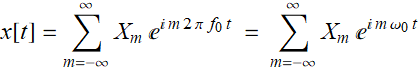
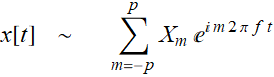
What is most remarkable is that the Fourier spectrum shows many peaks that have periodic spacing. It means that the sound signal can be written as:
                                            (1.1.1)
where f is the fundamental frequency found below:

and p are the number of peaks that are above the “fuzzy” noise floor.

Are those peaks are really regularly spaced? We can check by plotting:

1.2 Construction of the signal

Let’s use Eq. (1.1.1) to reconstruct the signal. Since the signal is over a long duration with some slight variation, we’ll choose a narrow interval as show below:

Over this range of signal:

Let’s look at the Fourier components:

Here are the Fourier component :

Now, we just apply the formula:
                                            (1.1.1)

One more thing: we don’t have to sum from -p to p like the equation says. Because the signal is real, we can just add the positive p components and take the Real part.

So, this is the synthesize signal:

Let’s plot our synthesized signal (yellow) to compare with the original (green):

Pretty close, given that we use a mere 9 components out of 515. This what they sound like:

2. Fourier’s theorem: an example

2.1 Discussion

Is it true that any periodic function can be expressed as a sum of harmonics with frequencies that are integral multiples of the fundamental frequency? Yes, that is exactly what Fourier’s theorem says,...

which means that we can represent a periodic function as a series, known as Fourier’s series
                          ;    (2.1.1)
where T is the period, and the Fourier series coefficient is obtained as
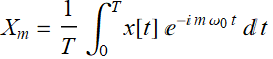                                                                            (2.1.2)

It is quite easy to construct a periodic function. All we have to do is to define it over one period, and repeat it. In programming language,we use modulo function so that the variable repeating itself after each period.

Consider as an example this simple function:
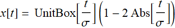            for t ∈[-0.5,0.5]
which can also be written as:
         

2.2 An example

2.2.1 Plot the function

2.2.2 Obtain Fourier coefficients

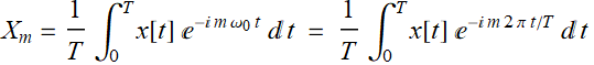
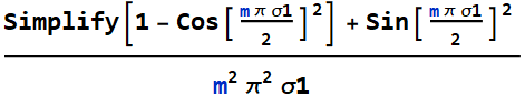
Let’s apply Fourier’s theorem to it. The Fourier’s theorem says first, we should obtain the coefficient:
                     

	0<σ1≤1 σ1>1 0 True

Hence, the Fourier coefficient is: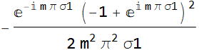  

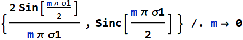
But we can simplify it a bit:

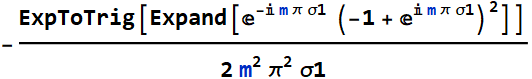
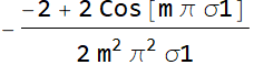
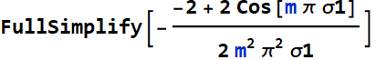
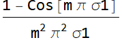
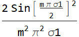
Hence, the Fourier coefficient is:

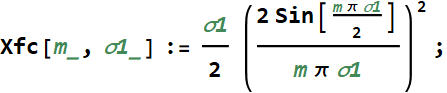
or

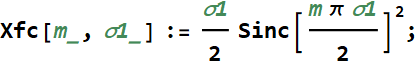
Why do we use Sinc function? just for this simple reason

2.2.3 Apply the Fourier’s theorem numerically

Code

3. Fourier signal synthesis

Can we use Fourier’s theorem to synthesize a signal? Certainly!

3.1 Example 1: signal synthesis concept

3.2 Example 2

4. Basic concept of Fourier analysis for a LTI system

A periodic signal can be decomposed into a sum of its Fourier components

With known system response, we know the output of each component. Remember this?

All we have to do is to add them up! See illustration below

4.1 Illustration of passive RC with Bode plots

4.2 Illustration of passive RC with Fourier analysis

To be continued to Part 2 - Fourier integral transform