Lect_3340_Fourier_background_review

Fourier Transform and Applications
- Part 2

ECE generic Han Q. Le (c)

(continued from Part 1)

5. The Fourier Integral

5.1 Concept

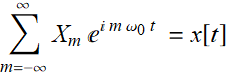
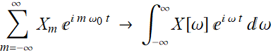
Consider a periodic function of period T, if T→∞, what would become of the sum
? (5.1.1)

First, let’s take a look of a typical example, suppose we have a square wave as shown below:

Code

Increase the period and we note that becomes very dense, for the simple reason: the fundamental frequency becomes very small: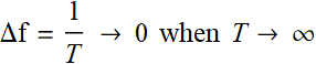
We observe that all the points of Fourier coefficients appear to morph into a curve. What kind of curve is that? We’ll see that it is known as the Fourier transform.

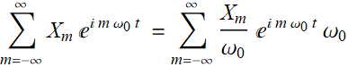
When we sum a function over a very dense sets of points, it approaches to an integral:
(5.1.2)
To be correct, we have to include the integration interval as well, right? Take a look at this:

As illustrated with the bar chart above, to express the concept of (5.1.2) rigorously, we write:
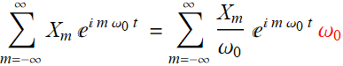(5.1.3)
where is the whole area of bar , we define 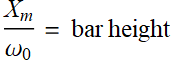, is the bar width, which will play the role of interval Δω in the integral. The interval is , which is . So, indeed, as T→∞, the interval as would be in an integral.

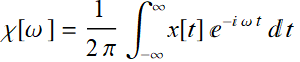
We define , then:
, and we define a function χ[ ]  such that:
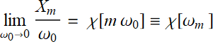                                                                        (5.1.4)
Then, Eq. (5.1.3) becomes:


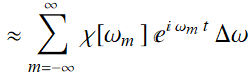
                                                                                              (5.1.5)
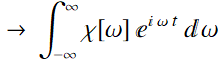
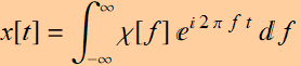
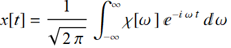
This means that we can express the input signal as:
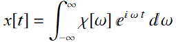                                                                                         (5.1.6)
and we refers to x[t] as the Fourier transform of χ[ω].

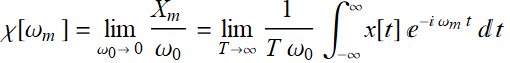
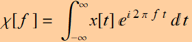
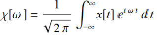
Conversely, we note that:
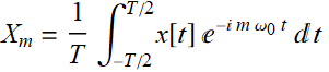                                                                        (5.1.7)
Let , then:


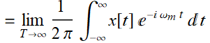
Dropping the dummy subscript m:
                                                                                    (5.1.8)
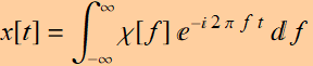
Thus, the pair of functions x[t] and χ[ω ] are referred to as Fourier transform of each other. Notice that there is a 2π factor involved. We can avoid this factor if we integrate vs frequency f instead of ω. Then:
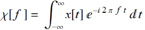                                                                                     (5.1.9a)
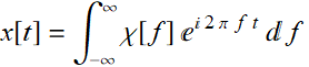                                                                                       (5.1.9b)
We also write symbolically:
                                                                                                          (5.1.10a)
and                                                 x=F[χ]                                                       (5.1.10b)
where F denote the Fourier transform and denotes the inverse Fourier transform. Not every function has a Fourier transform: for example function that diverges at infinity or does not vanish sufficiently fast at infinity: the integral value simplies does not exist.

One very important note: In the following, sometimes we will write:
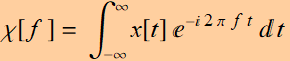                                                                                     (5.1.9a)
                                                                                       (5.1.9b)
and other times we will write:
                                                                                      (5.1.11a)
                                                                                     (5.1.11b)
There is absolutely nothing wrong with either way. Functions χ[f ] and x[t]  are not any specific functions and the equal sign doesn’t represent an equation, but a definition: the left hand side is always considered as a definition by the right hand side. In computer analogy, the equal sign is not == but only an assignment: = .

The reason we use (5.1.9) is that it is a continuation from our discussion of extension of Fourier’s theorem of periodic function to Fourier transform. For (5.1.11), we simply define the left hand-side by the right-hand-side operation.

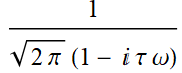
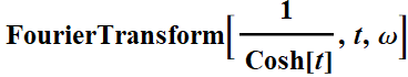
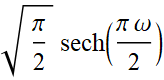
5.2 Example 1

What is the Fourier transform of this function?

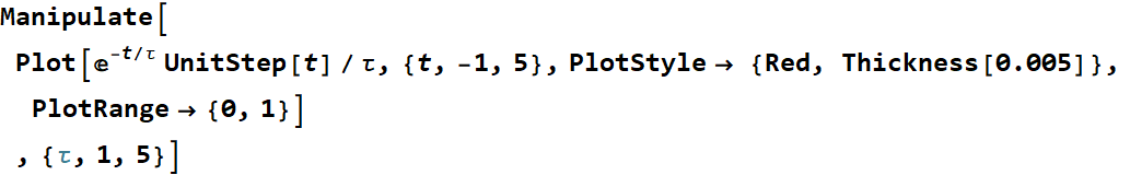
(drop the )
put back

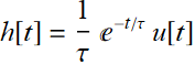
Recall that this was also how we could obtain the frequency response function:

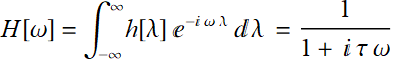
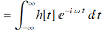
We have applied Cauchy’s integral theorem to obtained the Fourier transform:

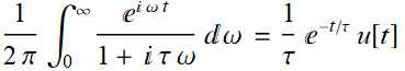
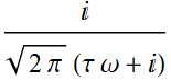
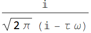
What is the Fourier transform of this function:
?

We notive that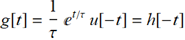
Then: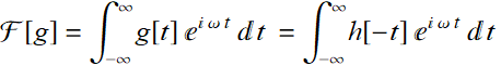

Since: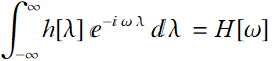
Hence: 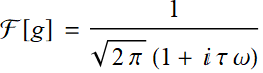                       (put back )

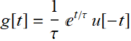
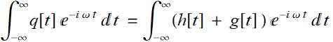
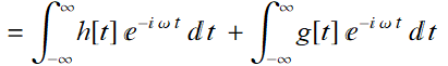
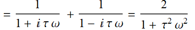
What is the Fourier transform of this function:

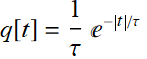
We notice that                             q[t]=h[t] + g[t]

5.3 Example 2

Find the Fourier transform of a square pulse: Π[t;a]

Code

Thus: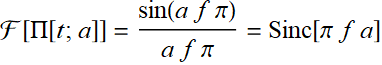
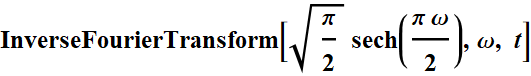
We can find the inverse Fourier transform:

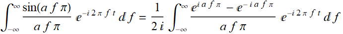
Apply Cauchy's integral theorems to find the inverse Fourier transform of
Remember this case and this:

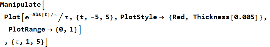
5.4 Other simple functions

Below is a graphic representation of common signal shapes and their Fourier transforms.

There are two interesting functions in the app, for which the Fourier transform of each is itself.

And Gaussian:

5.5 Another graphical illustration

5.6 Note on Fourier transform convention

There isn’t a unique definition of Fourier transform. The most common definition is:
(5.6.1)
amd the inverse Fourier transform for this case is:
(5.6.2)
The advantage of this definition is that it is symmetric with respect to the 2 π factor. However, there are other definitions of Fourier transform: see Mathematica note for other definitions of FT, which uses the definition above as the default. To use any other particular convention of FT with Mathematica, use this formula:

.
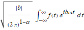with appropriate choice of FourierParameters a and b. Some common choices for {a,b} are {0,1} (default; modern physics), {1,-1} (pure mathematics; systems engineering), {-1,1} (classical physics), (signal processing).

6. An empirical view of Fourier transform

When you see this...

You are actually looking at a case of Fourier transform.
Later you will see that when we use our eyes to look at something, Fourier transform already happens twice to help us seeing it. The purpose of this section is move beyond the perspective of Fourier transform as an abstract mathematical entity. It is anything but abstract in the physical world and this is the view now that we will learn.

6.1 Example of sound:

Consider this sound:

Are there three different sounds? What sound is - physically- is just an air pressure wave hitting our eardrum, but what is the property of the air pressure that we can tell they are different?

Code

We can guess from the illustration above: the rate of vibration of our eardrum is different for each sound, which is what we call “frequency”. But mathematically, how do we express this difference? As it turns out, the most mathematically elegant way to see the difference is to take the Fourier transform of the vibration of our eardrum, this is what it shows:

eardrum vibration

Fourier transform

1st sound note

2nd sound note

3rd sound note

The left hand side x-axis is time (in millisec). The green plot represent the eardrum position vs. time. We can see they are different somewhat for the three sounds. But what is far clearer and definitively more elegant to show the sound difference is the right hand side, the Fourier transform. The x-axis of the FT is 1/time, which is what we call frequency (in unit of Hz).

Not only the Fourier transform graphs are much clearer with sharp peaks, it is also very clear that each sound has a distinctive set of frequencies. Each sound has a regular-spaced pattern of frequencies, and the frequency spacing is the single most definitive determinant feature that distinguishes the three sounds. This is what we say the sounds have different “pitches.”

Fourier transform is not just an abstract mathematical entity for curiosity and amusement, in this course (or generally in science and engineering), it is the natural language to describe certain aspects of the natural world: in fact, perhaps the most fundamental phenomenon of nature as we know it: the wave phenomenon.

6.2 Concept of domain

When we look at the formula: ,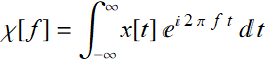
it appears abstract. Variable t is just an element of the Real number domain: t∈R, and so is variable f of the FT: f∈R. But in the context of applying to describe nature, t and f could not be more different: They have to have the unit of being inverse of each other so that their product is unitless and is physically meaningful.

In the example above, t is time and f is frequency in unit of 1/Time. They don’t belong to the same Real number set R like in pure math. They belong to different domains: time domain and frequency domain.

But is that the only domain pair in nature? No. Generally speaking, given any domain with variable var with a real physical meaning, its Fourier transform is in the 1/var domain, and we call them a domain pair: {var, 1/var}. Besides time, what else is a fundamental physical domain? you guess it, space, and the domain pair here is {space, spatial frequency}.

6.3 An example of Fourier in spatial domains: Fourier optics

Not only our sense of hearing involves Fourier transform, which is in the time-frequency domain, even more so is our vision -and perhaps more interestingly, this involves the space-spatial frequency domain. And this is not just about our human-specific vision, it is the fundamental behavior of waves, from EM waves to gravitational waves which involve the Fourier transform of space.

Wave is a phenomenon that ties space and time together. As we have seen in other lectures, the most fundamental property of a wave is that it progagates, and hence, the most fundamental parameter is the speed. If a wave is fundamental of nature, so must be its speed. Hence, space and time are not independent because they have to be tied together such that it is the speed that is constant. As of now, the speed of light (EM waves) and gravitational wave is a constant of the Universe as we know it:

exactly.

Hence, the mathematics of Fourier transform when applied to nature is not just for time, but also for space, and our eye is a beautiful illustration of it.

Have you ever wonder why the real image projected by a lens is inverted, like those shown below?

The reason is best described with Fourier transform: the image is inverted because it is two-time Fourier transform. When light propagates, it actually performs Fourier transform of itself.

Light scattered from an object, e. g. the tree in the picture above propagates as a Fourier transform of the scattered light (image of the tree) but with a nagging extra term: the quadratic (and higher order) term of phase known as Fresnel term.

What the lens does is something remarkably simple and beautiful: it negates the Fresnel term, restoring the original image of the object in the subsequent Fourier propagation, known as Fraunhoffer diffraction. But the Fourier transform is applied twice: from the object to the front of the lens, and from the back of the lens to the image plane.

... and the image is inverted because of being twice-Fouriered!

Guess what left pict in the title of the lecture show?

Yes, it is Fourier being Fouriered.

6.4 Examples of spatial Fourier transform: diffraction

6.4.1 Concept of diffraction through an aperture

Watch the video below. See what the waves do after getting through the seawall aperture.

What it does is called “diffraction”. This happens to EM waves also. Below is the light diffraction case.

6.4.2 Fraunhofer diffraction

6.5 Examples of 2D spatial Fourier transform: images

6.5.1 Image 1

Consider this picture of a building with windows.

image	Fourier transform

Do you notice some relationship of left and right?

Take a look at the Fourier transform of the below:

image	Fourier transform

We don’t see a regularly-spaced pattern here like that of the window image.

6.5.2 Image 2

Consider this image:

image	Fourier transform

Notice something about the relationship between the two? See below with X-ray and electron diffraction of crystals.

6.6 How Fourier transform helps discovering nature - example 1

Excerpted:
A Structure for Deoxyribose Nucleic Acid. Watson J.D. and Crick F.H.C. Nature 171, 737-738 (1953)

Molecular Structure of Deoxypentose Nucleic Acids. Wilkins M.H.F., A.R. Stokes A.R. & Wilson, H.R. Nature 171, 738-740 (1953)

Molecular Configuration in Sodium Thymonucleate. Franklin R. and Gosling R.G. Nature 171, 740-741 (1953)

6.7 How Fourier transform helps discovering nature - example 2

Not only one can measure the dimension of ultra-small structure like a crystal, it demonstrates something fundamental: the quantum-mechanic wave behavior of particles, of which the propagation is also best described with the mathematics of Fourier transform.

The single most important material in today Information-Communication Technology industry:

The right most is the Si crystal diffraction image, which is proportional to the Fourier transform of its spatial crystal structure.

Crystal material science and technology would not have been what it is today without the indispensible tool of X-ray and electron diffraction that are most naturally described with the mathematics of Fourier transform.

Created with the Wolfram Language