 \
\
Fourier Transform and Applications
- Part 3
ECE generic Han Q. Le (c)
\
(continued from Part 2)
7. Properties of the Fourier transform and related theorems
7.1 Real and Imaginary part:
Consider: 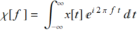 (7.1.1a)
1. If x[t] is real, then: 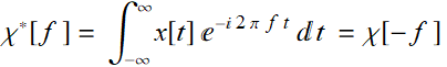 (7.1.1b)
2. We can take the Re and Im part:
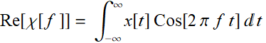 (7.1.2a)
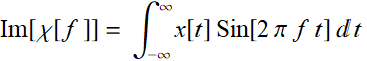 (7.1.2b)
We notice that, because of the even and odd property of Cos and Sin function:
 (7.1.3)
Hence, Re[χ[f ]] is even, and similarly, Im[χ[f ]] is odd.
3. If x[t] is even, then Im[χ[f ]]=0, or χ[f ] is purely real
4. If x[t] is odd, then Re[χ[f ]]=0, or χ[f ] is purely imaginary
Since generally:  (7.1.4)
The Fourier transform:
![]() (7.1.5)
(7.1.5)
is a general complex number (neither purely real nor purely imaginary, and thus, the phase of a Fourier transform is related to the function asymmetry. But this symmetry depends on the origin. For example:
Illustration
We see that just by translating the signal function away from the origin, the 3D line of the FT twists away from the real axis plane. The added phase ![]() is meaningless unless there are other signals and their relative phase differences are important.
is meaningless unless there are other signals and their relative phase differences are important.
We’ll see in Section 7.3 that the phase is also related to relative position of the signal or parts within the signals. An example of the importance of the phase term is wave diffraction of periodic structures.
Illustration 1: Diffraction grating or the CD/DVD/BluRay effect
Illustration 2: phased array antenna:
The relative phase differences between the dipoles determine the bearing, i. e. azimuthal angular direction of the main lobe of the radiation.
7.2 Delta function and Fourier transform
What is the Fourier transform of delta function? We know that delta-function is not a conventional function, but if we apply the formalism:
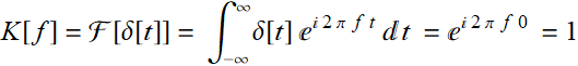 (7.2.1)
This is not qualified as true Fourier transform, since the function K[f]=1 is not integrable from -∞ to ∞ and we cannot obtain the inverse transform:
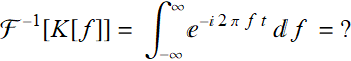 (7.2.2)
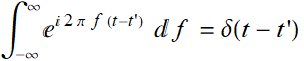
It is indeterminate. However, if t≠0 and if we make the convention that:
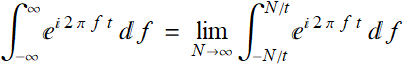
then:
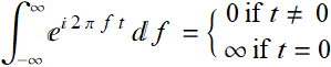 (7.2.3)
which is a property of δ-function. We still need the property:
 (7.2.4)
for 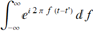 to act like δ(t-t') .
Let's look at Eqs. (5.1.11a and b) above:
 (5.1.9a)
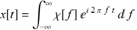 (5.1.9b)
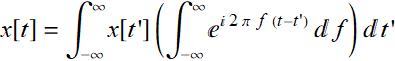
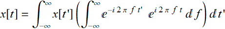
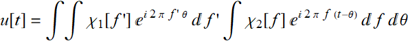
If we take χ[f ] in (5.1.9a) and insert in (5.1.9b), we obtain:
 (7.2.5)
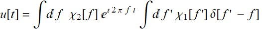
Rearranging (7.2.5):
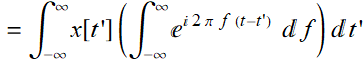 (7.2.6)
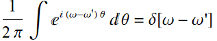
But we recall that:
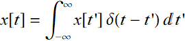 (7.2.7)
Thus, Eqs. (7.2.3) along with (7.2.6) allows us to conclude:
 (7.2.8)
Obviously, it is only a convention, but we'll see it can be very convenient. It is obvious by taking the conjugate that (7.2.8) is valid for both +f or -f in the exponent of the left hand side.
7.3 Fourier Transform Theorems
There are a number of basic properties of FT that are straightforward. Knowing these theorems sometimes can help to find FT without too much work. These are: (in the following, we denotes χ[f] as the FT of x[t], or F[x])
1. Linear superposition:
![]()
![]() (7.3.1)
(7.3.1)
2. Translation or time delay
![]() (7.3.2)
(7.3.2)
3. Scaling
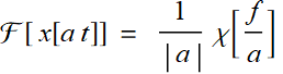 (7.3.3)
A special case is reflection or time reversal:
![]() (if real) (7.3.4)
(if real) (7.3.4)
4. Duality:
F[ χ[t]] = x[-f] (7.3.5)
(this is related to ![]() )
)
We have discussed a beautiful illustration of this simple theorem:
5. Frequency shift (translation): (follow from 2 and 4)
![]() (7.3.6)
(7.3.6)
A special case for amplitude modulation:
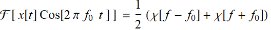 (7.3.7)
From an app in Part 2:
We see that with a carrier, the Fourier transform of the signal (a ramp in this case) consists of two components centering around ![]() and
and ![]()
6. Differentiation:
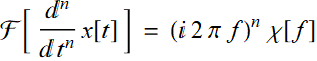 (7.3.8)
7. Integration:
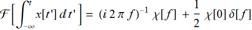 (7.3.9)
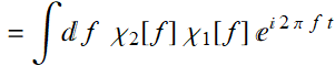
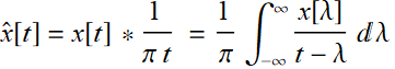
8. Convolution: (remember this)
![]() (7.3.10)
(7.3.10)
9. Multiplication: (this follows from 8 and 4 above):
![]() (7.3.11)
(7.3.11)
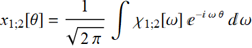
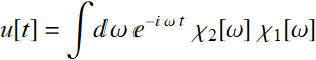
7.3.1 An additional note on convolution
Note that the theorem on convolution does involve the Fourier parameters of a given convention of Fourier transform. The above theorem is appropriate when we use the signal processing convention.
Let 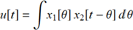 (7.3.12)
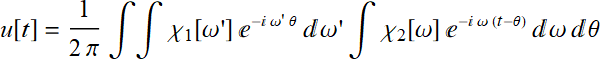
We substitute: 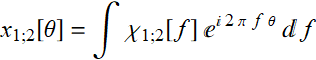

Since: 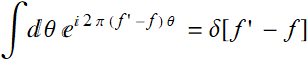
Thus, it is obvious that:
![]() (7.3.13)
(7.3.13)
The reverse can be similarly proven.
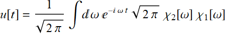
However, we should note that for other convention:
 (7.3.14)
The result is:
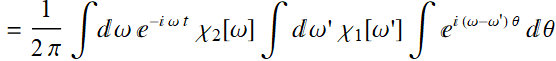
Similarly to the above:
Hence:
Thus: ![]() (7.3.15)
(7.3.15)
We see that there is this factor ![]() that may appear a bit odd, but it is just a factor and does not really affect anything fundamental about this theorem. In fact:
that may appear a bit odd, but it is just a factor and does not really affect anything fundamental about this theorem. In fact:
![]() (7.3.16)
(7.3.16)
![]()
Or: 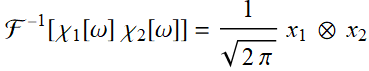 (7.3.17a)
Collorally: 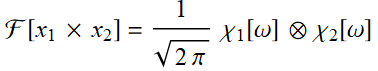 (7.3.17b)
As long as the coefficient is kept consistently, it will work out fine.
7.4 Generalized functions
We have seen FT of delta function. The following are the FT of generalized functions, which are useful when FT is applied to power signals (instead of only energy signals).
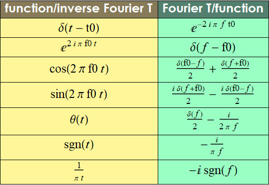
7.4.1 Most common functions
| function/inverse Fourier T | Fourier T/function |
| DiracDelta[t-t0] | |
| DiracDelta[f-f0] | |
| Cos[2 f0 π t] |  |
| Sin[2 f0 π t] |  |
| HeavisideTheta[t] | 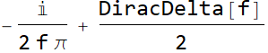 |
| Sign[t] |  |
| -i Sign[f] |
In traditional format: (7.4.1)
In addition to these results, two other related FTs also useful in many applications are Hilbert transform and periodic delta-function sampling waveform or ideal sampling waveform (or impulse sampling waveform).
1- Hilbert transform is defined as:
 (7.4.2)
The FT of ![]() is:
is:
 (7.4.3)
2- An ideal sampling waveform is simply a periodic delta-function: 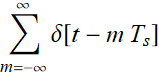 . We have studied this in Chapter 3, Lecture 3-2:
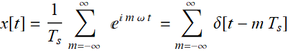
Its FT is simply: 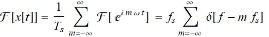
or:
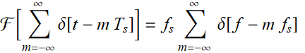 (7.4.4)
8. Power and Energy Spectral Density
8.1 Introduction
See the ppt part of the lecture.

Link to ppt on the concept of spectrum
8.2 Discussion
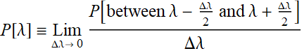
Consider the figure above, suppose we have a solar cell that works from 400 nm to 800 nm and want to know how much sun power it can generate, we start by finding out how much total sun power in that wavelength range:
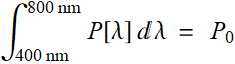 (8.2.1)
where P]λ] is sunlight power as a function of wavelength. Since ![]() is power, in unit of, say, watt, then function P[λ] has to have the unit of watt/(unit of wavelength). Thus, P[λ] is the power per unit of spectral wavelength, or we can just call it “power spectral density”:
is power, in unit of, say, watt, then function P[λ] has to have the unit of watt/(unit of wavelength). Thus, P[λ] is the power per unit of spectral wavelength, or we can just call it “power spectral density”:
 (8.2.2)
8.2.1 Example of discrete spectrum
Now, let’s consider a voltage signal, like this:
that is applied to our 50-Ω load. What is the power delivered to the load? For instantaneous power, it is:
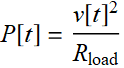 (8.2.3)
and more relevant is the average power per unit of period:
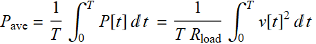 (8.2.4)
For simplicity, from now on, we will drop ![]() and treat it as 1 because it is just a constant factor.
and treat it as 1 because it is just a constant factor.
There is another way to look at power: we have learned from Fourier’s theorem:
| signal | First 4 non-dc components |
|
 |
Fourier→ |  |
| power | harmonic power | |
 |
 |
As shown above, we know that each real harmonic component ![]() delivers an average power:
delivers an average power: 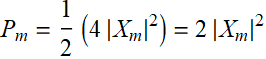 (8.2.5)
then, the total power average power for all components should be:
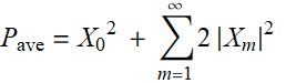 (8.2.6)
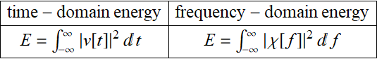
If so, these two expressions of power should be equivalent:
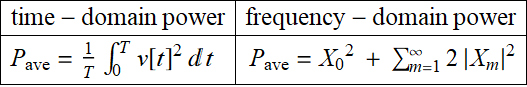 (8.2.7)
which is Parseval’s theorem that was covered in Chapter 3.
| time domain power |
 |
|
| frequency domain power |
 |
 |
In the above, we see that power can be expressed as a function of frequency, this is the concept of spectrum: power vs. frequency. In this case, the spectrum is discrete because the frequency set is.
8.2.2 Example of continuous spectrum
However, what if the signal is only one pulse:
The concept of instantaneous power still applies, but over the whole pulse duration, or over all time from -∞ to ∞, assuming that the pulse has only finite duration as shown, the key concept is total energy delivered to the load:
 ;
; 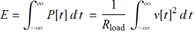 (8.2.8)
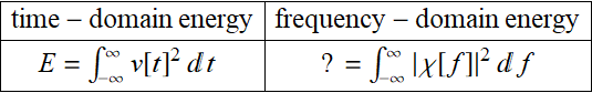
What becomes to the Fourier transform?
| signal | Fourier transform | |
 |
Fourier→ |  |
| instant. power / total energy | harmonic power / total energy | |
 |
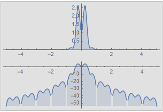 |
In fact, for the FT, frequency variable f simply becomes continuous. The absolute square of the FT, ![]() must be somehow proportional to the power or energy density of the harmonic associated with f. In this case, we have a continuous spectrum, and instead of a sum, we have an integral:
must be somehow proportional to the power or energy density of the harmonic associated with f. In this case, we have a continuous spectrum, and instead of a sum, we have an integral:
 (8.2.9)
8.3 Parseval’s theorem extension to continuous variable
In Chapter 3, lecture 2, we have learned about Parseval’s theorem for the Fourier series of a periodic function and we mention it again in 8.2.1 example above. Now, let’s take a look at the case of continuous signal.
If a signal is square integrable from -∞ to ∞, i. e.
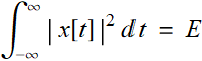 (8.3.1)
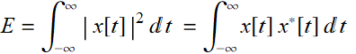
then, we define it to be an energy signal. For the sake of generality, we will allow x[t] to be complex and if it is associated with a real physical quantity such as voltage, then, like phasor, we’ll let the physical quantity be its real part. If the signal has a Fourier transform, we can substitute to see that:
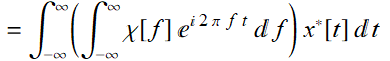 (8.3.2)
Re-arranging:
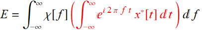 (8.3.3)
We notice that:
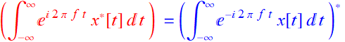
![]() (8.3.4)
(8.3.4)
Substitute (8.3.4) in (8.3.3), we obtain:
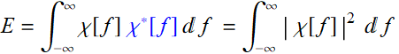 (8.3.5)
Comparing (8.3.5) to (8.3.1), we see that:
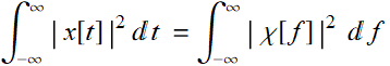 (8.3.6)
Thus, we have Parseval's theorem for the continuous FT and we can assert the case above:
 . (8.3.7)
The function
![]() (8.3.8)
(8.3.8)
represents the energy density per unit of frequency, and we call it energy spectral density. From the pure mathematics perspective however, x[t] can be anything, even variable t needs not be time. If so, why would we use concepts like energy and power as energy per unit time? The answer is simple, it is just a convention.
8.4 Empirical applications and examples
Recall that when we discussed Bode’s plot, we mentioned that who would ever be interested in Bode’s plot for a system with a perfectly known analytic model? It is the empirical Bode’s plot for an unknown system that we want to understand and discover is what make it interesting.
The same can be said to PSD function: the reason we learn it is to apply to data of systems or subjects we want to study. As shown in the ppt files, there are numerous applications of PSD functions. Below, we do a few more and some more in HW.
8.4.1 Sun spots
Consider this example:
This is a phone ring tone of 10 x sun spots data
What is its power spectral density? Notice how funny the units are: for frequency, instead of Hz (1 per second), we have ![]() or per year. Since the data is monthly, we have max Nyquist frequency of twice a month of 6/year. For the vertical scale, the unit is (ahem...)
or per year. Since the data is monthly, we have max Nyquist frequency of twice a month of 6/year. For the vertical scale, the unit is (ahem...)
![]()
What does it show? First, the 11-year cycle is obvious, and there is a weak 2nd harmonic. But does it appear to have a shorter cycle of 10 year (frequency 0.1/per year) and a long cycle of 0.0112 or ~ 89 year period?
 |
 |
A way to analyze is to plot those components which we will do in HW. For the 89-year component, is it real? Given that the data is only 2.5 century, a cycle of almost a century is statistically meaningless.
But quite interesting is the high-frequency tail of the spectrum. It almost looks like /![]() noise, α could 1 or slightly less than 1, and the 1/f noise is as it should be since the sunspots must be related to some internal process that has a cause-and-effect correlation of its past.
noise, α could 1 or slightly less than 1, and the 1/f noise is as it should be since the sunspots must be related to some internal process that has a cause-and-effect correlation of its past.
8.4.2 Gold price , Bitcoin price, and others
See the following results: (all the data below are from FRED server of the Federal Reserve Bank of St. Louis)
https://fred.stlouisfed.org/
The left hand sides are the price (top) and the relative price change (bottom). Their correspondent power spectral densities are on the right. Below is for gold daily price.
 |
 |
 |
 |
This is for Bitcoin
 |
 |
 |
 |
Besides the remarkable market psychology parallelism between price and bitcoin (both have peak mania and subsequent correction crashes), the PSD tell a fundamental market law. There cannot be any periodicity of the market price daily change, because if so, the price change is predictable and the market would quickly exploit it, destroying any periodicity. Indeed they all obey double-sided Laplacian distribution and the fluctuation is a Brownian process.
For the price, if the price change is Brownian, it must obey the “drunkard random walk down Wall Street” law and its PSD exhibits 1/f behavior, perfect to a t.
This economic market behavior - based on human trading behavior, is as fundamental and immutable as physical laws or more precisely, human economic genetic behavior. It applies to stock prices, ...anything involving human trading bahavior. Below are the prices of two items as different from gold and Bitcoin as possible, yet the same law applies:
 |
 |
 |
 |
 |
 |
 |
 |
Notice however, there are big differences in the PSD magnitude: the fluctuation of Bitcoin price certainly demonstrate a much high volatility than something as low-risk as US T-bill or something as efficient a commodity as oil.
8.4.3 Earth temperature data from Vostok ice sheet
This is for HW
8.4.4 US consumer behavior
This is for HW: analyze the PSD of VMT in the US.
Should there be any similarity in the PSD of US gasoline consumption and that of vehicle miles traveled?
Driving behavior and gasoline consumption in the US are driven by economic and cultural activities as well as seasonal effects including the weather condition (more in summer, less in winter, occasional peak on Thanksgiving etc.). Regardless of oil price, people will do what they do. But is there any price elasticity? It is NOT just about the absolute gas price because surely, if the price is above $4/gallon, many will drive less - as it can be seen in those oscillations when the price hit $4/gallon 2011-2014. But more interesting is whether the price change, e. g. 20% increase or decrease would have people to drive slightly more or less? We may also notice that the price tends to go up during Thanksgiving etc. The topic we’ll learn later is regresssion and time-series data correlation that can handle these questions best. However, it is worthwhile for us to look at the PSD to see if there are any interesting features there.
8.5 Empirical-data-based formulation
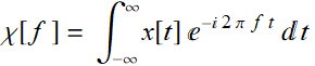
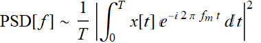
For all the emprical examples above, it is obvious that we could not have obtained the PSD ![]() via Fourier transform in the strict mathematical sense:
via Fourier transform in the strict mathematical sense:
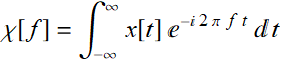 (8.5.1)
First, in reality, there is no such a thing as a signal known from -∞ to ∞. The data is available only over some duration T, let’s say from -T/2 to T/2. Then, we can only do this:
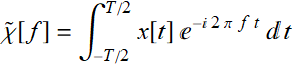 (8.5.2)
and define conceptually:
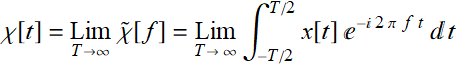 (8.5.3)
In other words, the more data we obtain of signal x[t], the more accurately does function ![]() approximate the true value χ[t].
approximate the true value χ[t].
However, there is a problem with (8.5.2): what it does, is this:
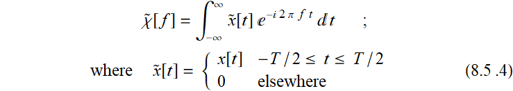
In other words, it is the Fourier transform of a truncated signal function. Is this correct? Suppose we measure the sun spots like the above example and have data only for 2.5 centuries, should we use a formalism that implicitly assumes the sun spot number was zero before the data is collected and zero afterward for billions of years to come as long as the sun still lives?
A more logical way to handle this (and we’ll see later a natural consequence of DFT) is that we should just pad the data before and after with the same data we have from -T/2 to T/2. In other words, treat the data as a periodic function with a super long period of T. Then, instead of (8.5.2), we should use the Fourier series component:
 (8.5.5)
with the Fourier component power:
 (8.5.6)
such that Parseval’s theorem can be applied:
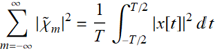 (8.5.7)
What is essential of Eq. (8.5.7) is this:
 (8.5.8)
Hence, regardless what T is, whether we observe the sun spots for 5 years for 5 million year, the result of (8.5.8) is still a measure of the true, intrinsic value of the average power of the quantity of interest. The only difference between large-T data and small-T data is about the accuracy and uncertainty, not about the magnitude of the quantity to be measured. In other words, if we measure something with a definite invariant value, we can measure it 5 times or 5000 times to take the mean, it is still the same value that is measured and only the uncertainties of the results are different.
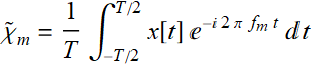
Hence, based on (8.5.7), we can use the same approach when we discuss continuous Fourier transform in as the case discussed in Section 5.1: we define for the left hand side of (8.5.7):
 (8.5.9)
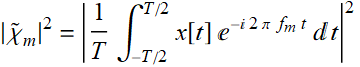
The empirical-based definition of power spectral density is thus:
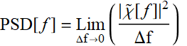 (8.5.10)
where we drop the dummy subscript m from ![]() .
.
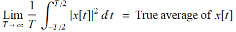
A more practical expression of (8.5.10) using Eq. (8.5.7) and replacing Δf→0 with T→∞:
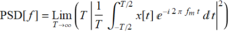 (8.5.11a)
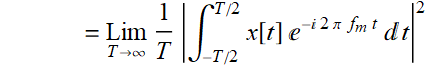 (8.5.11b)
This is exactly the formula we used in all the examples of this chapter, including those in Section 8.4, and in all the software utility packages associated with the Fourier series lecture.
8.6 An introduction to noise power spectral density
It may appear that what we learn in this chapter is interesting only if applied to periodic phenomena. That’s actually not true. Power spectral density is also useful to study noise phenomena, especially when noise affecting periodic phenomena of interest. In all electronic devices, noise power spectral density is an important figure of merit, as shown in the example below:
The high-lighted figure above is about voltage noise, not voltage noise power, hence, instead of the unit:
 ;
;
the spec sheet shows 
A spec sheet typically shows the ![]() for the user to consider in circuit design. Below shows the voltage noise spectral density and the current noise spectral density for the op amp above.
for the user to consider in circuit design. Below shows the voltage noise spectral density and the current noise spectral density for the op amp above.
And this shows that not all noises are the same: low frequency noises in the 1/f-characteristic range must be handled differently from high-frequency noises which appear to be flat, or “white-noise” in the above. What does this mean to a user? A user who designs for example, some applications in certain frequency range, e. g. few Hz must be aware of the noise level at that range, which is higher than the noise level for 100 Hz and above.
As a simple example, if a user uses it for a robot with a control operated in the range of few Hz, it is not wise to send/receive the control signal at the baseband, but to modulate the control signal with a higher carrier frequency, e. g. 100 kHz for lower noise, and then demodulate to obtain the baseband signal. Thus, noise spectral density is a very important figure-of-merit.
How is the noise measured to be reported in this spec sheet? Exactly by the approach we just learn above:
except that T doesn’t have to be approaching to ∞, but just a few times longer than the lowest ![]() show, which means just a few seconds shoud suffice.
show, which means just a few seconds shoud suffice.