Generic ECE-3340 supplementary note: Polynomials
                                                                 (c) Han Q. Le

1. What is a polynomial

2x+1 ;  x is a variable. It is a polynomial of x.

; x and c are constant (can be unknown), q is a variable. Then it is a polynomial of q

is a polynomial of x and y if both are variables.

In[4]:=

Out[4]=

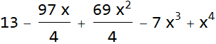
2. For a single-variable polynomial, what are the most fundamental parameters

Consider:           
Are coefficients 4,        28,      69,      -97,      52
the most fundamental parameters of the polynomial?

No. It is this:

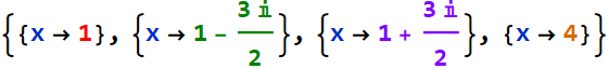
It is the zeros or roots that are fundamental to a polynomial. We construct a polynomial from the roots (up).

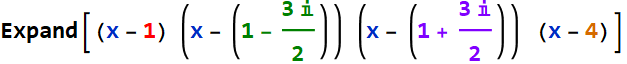
We need just a proportional constant:

Hence:

For a real-coefficient polynomial, the fundamental way to express it is:
                     
where are a pair of conjugate roots, and , are real roots.

3. Linear system transfer function

In this course, the reason we are interested in the polynomial is that it can be used to represent the Laplaced-transformed response or transfer function of a linear system.
(please review course materials of circuit analysis, signal analysis, or signals and systems)

What determines the behavior of these circuits or linear systems? The roots (or poles) of their Laplace transfer/response functions.

3.1 Example 1:

Please go to this website to watch the behavior of second-order circuits as functions of the Laplace TF poles.

http://courses.egr.uh.edu/ECE/ECE3340/Class%20 Notes2100/Lab_6/ECE2100_Lab6_v2 _p1.htm

Read additional notes about filters.

3.2 Example 2: Allow the shockwave flash video to see.

3.3 Example 3:

Discussion of PID controllers.

4. Example of coding for transfer functions

4.1 Usage of Product function

In general, a transfer function can be written as:
             
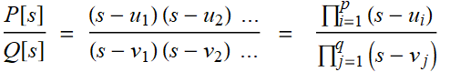
where , i from 1 to p and , j from 1 to q are the roots of the numerator and the denominator.

The mathematical symbol, 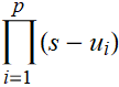is known as “product” and it can be used directly in Mathematica code:

To explicitly spell out the function without using the symbol, we can write:

Hence, suppose we have a list of roots, we can easily construct the TF programmatically. Below is an example.

4.2 Example 1

Suppose we have a list of desired , we first define function for the roots:

What if it is a single real root? then we just use the root directly. So let the list of single real roots and   be:

What would be the polynomial? First, we get the root pairs:

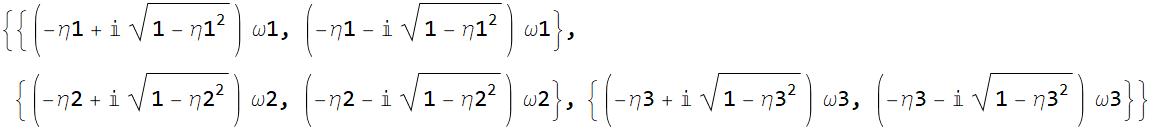
The dimension above indicates that rootpr is a 3x2 array. But we want just a single list of 6. To do that, we need to flatten it by one level:

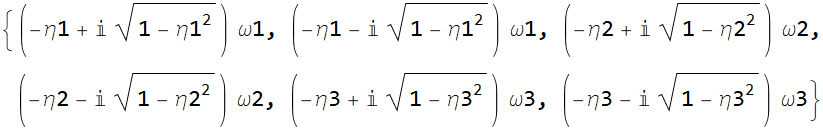
We see that it is just a list of 6 roots as expected. Now we are ready to construct the polynomial:

Let’s do a plot test:

Notice that we define the polynomial with formulated roots, but not numeric values. Yet, as soon as we assign numeric values to the various root parameters, Mathematica will substitute numerical values into those symbols and we can plot the actual function.

4.3 Example 3

This example is from HW3,
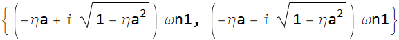
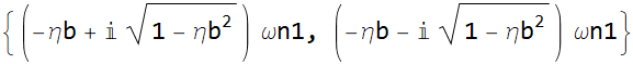
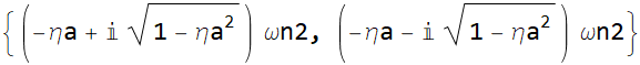
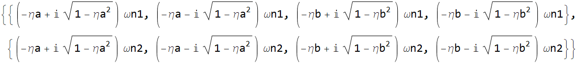
Let the lists of natural frequency and damping coefficient be:

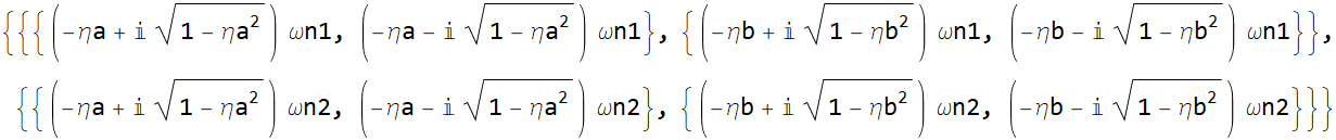
This is how you can see its structure:

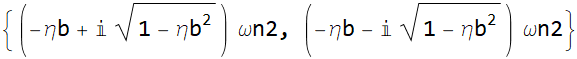We can define the top row, after flatten it as root1 and the second row is root2.

Now we can define the low-pass, hi-pass, and band-pass TF:

We can put all into a function:

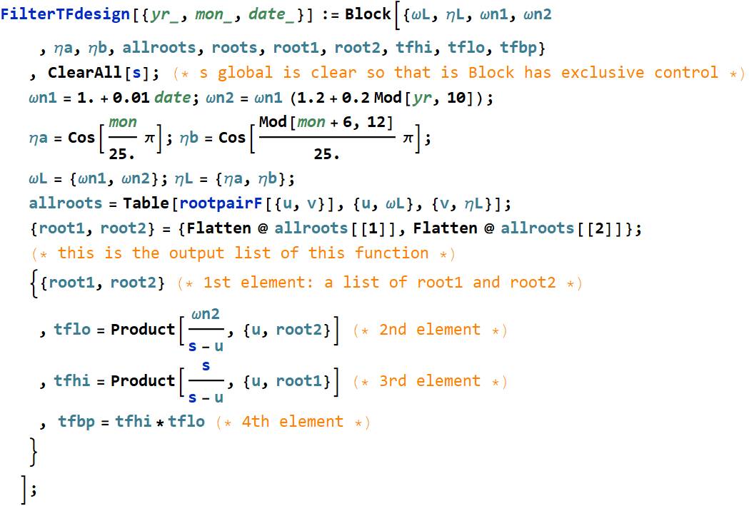
Example:

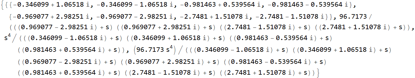
This is how to get the output: create variables to be used later:

Some additional functions that can be used in the HW:

Here is a test of the various functions developed: