
Tutorial 3 - Linear Algebra 1
generic ECE - U. Houston
Han Q. Le (c) copyrighted
1. Vector dot (inner) product
1.1 Example 1
Consider this data:
Out[10]=
| Trip category | A | B | C | D | E | F | G |
| # of trips | 5 | 2 | 6 | 3 | 3 | 1 | 4 |
| mileage/trip | 1052 | 740 | 576 | 1380 | 824 | 10850 | 438 |
Exercise 1.1
Define variable ntrip that contains data of the first row, and mileage that contains the data in the second row. Then find the total frequent-flyer mileage.
Answer

Out[13]=
![]()
END exercise
In the above, we see that any one-D array can be considered as a vector in space (linear algebra concept). The length of the array is the dimension of the space.
What we learn above with vector ntrip and mileage is their �dot product�, one of the MOST frequent and useful math operations of array data.
Consider this example: one has a number of shares of various stock shareX at priceX, what is the value of each stock and what is the net value?
In[27]:=

Out[28]=
![]()
Out[29]=
![]()
In[30]:=
![]()
Out[30]=
![]()
The dimension of the space of priceX is 4.
1.2 Dot product
The operation between 2 arrays:
![]() and
and ![]()
![]()
as mentioned, a most common operation in computer calculation of
arrays, is mathematically formally defined as the dot product:
![]()
where x array and y array are considered as
vectors.
In all higher-level language, using function dot means we can skip step in more basic language, such as using do loop:
In[1]:=

![]()

Out[4]=
![]()
The trend of computing is to create more and more built-in high-level functions such that the user can obtain results with less and less programming effort. Mathematica, Matlab, high-level library and special packages (R, Spyder) in Python, etc. are designed toward this goal.
Examples of dot product are abound and common in spreadsheet calculations. In fact, even the sum (total) of an array is considered as the dot product of the array and vector {1,1,1,...}.
Here is a common application:
In[34]:=

Out[37]=
![]()

Out[42]=
|
||||||||||||||||||||
|
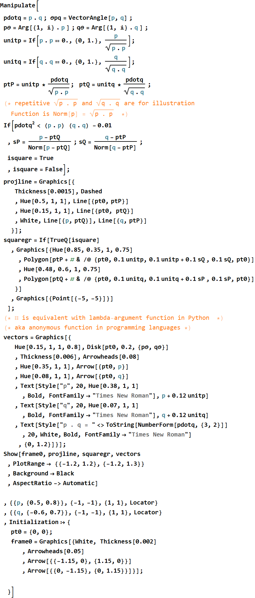
Below is what we learn about dot product between physical vector in 2 D space:
In[8]:=
Out[8]=
Exercise 1.2
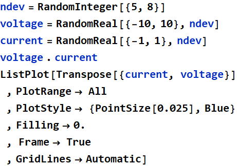
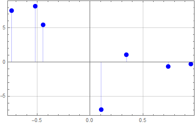
Consider a circuit with n devices, make your choice of n between 5 and 8. Generate arrays of the device voltages and currents (your choice of values). Find the net power consumption of all devices.
Answer
In[109]:=
Out[109]=
![]()
Out[110]=
![]()
Out[111]=
![]()
Out[112]=
![]()
Out[113]=
Exercise 1.3
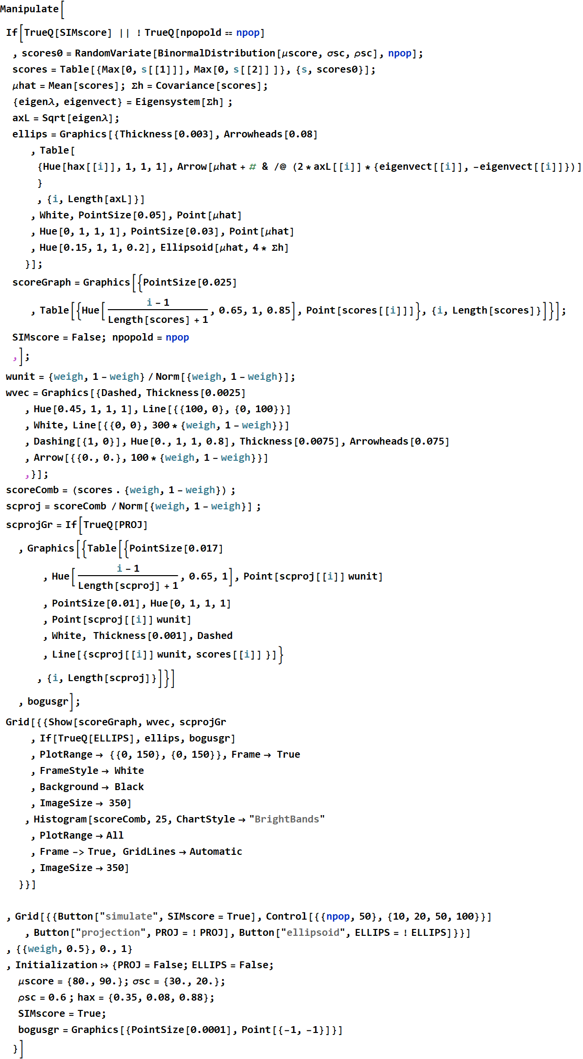
Consider the score of a student as a two-D vector:
{homework, classwork}. One way to combine this into a final score
is to assign a weight to each score, for example:
![]()
Generate a multinormal random distribution to simulate a class (e.
g. 100), and obtain a histogram of the combined score as a
function of weight
Answer (given)
In[141]:=
2. Matrix and vector product
2.1 Table of higher dimension: List of List
Consider this:
Out[8]=
| price($)/unit | |||||
| # units | store A | store B | store C | store D | |
| juice | 3 | 1.55 | 1.45 | 1.65 | 1.4 |
| eggs | 4 | 1.95 | 2.4 | 2 | 2.2 |
| fruits | 12 | 0.85 | 0.8 | 0.7 | 0.8 |
| vegetables | 8 | 1.35 | 1 | 1 | 1.1 |
| milk | 2 | 2.55 | 2.25 | 2.55 | 3.1 |
| cereals | 6 | 2.7 | 3.35 | 3.05 | 3.45 |
| coffee | 1 | 10.85 | 7.5 | 8.45 | 8.5 |
| tea | 2 | 4.2 | 4.15 | 3.75 | 3.95 |
| ice cream | 3 | 7.35 | 6.75 | 6.75 | 4.95 |
| napkins | 5 | 1.1 | 1.2 | 1.2 | 1.25 |
| foils | 2 | 3.5 | 3.75 | 3.6 | 3.75 |
| storage bags | 10 | 0.8 | 0.7 | 0.85 | 0.7 |
| toothpaste | 4 | 1.6 | 1.6 | 1.55 | 1.6 |
| shampoo | 3 | 3.55 | 2.6 | 2.9 | 2.7 |
| detergent | 2 | 9.55 | 9.05 | 8.65 | 7.1 |
How do we represent such data? It is a table. The first row is just
![]()

In[68]:=
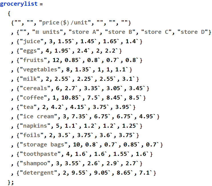
In[69]:=
![]()
Out[69]=
| price($)/unit | |||||
| # units | store A | store B | store C | store D | |
| juice | 3 | 1.55 | 1.45 | 1.65 | 1.4 |
| eggs | 4 | 1.95 | 2.4 | 2 | 2.2 |
| fruits | 12 | 0.85 | 0.8 | 0.7 | 0.8 |
| vegetables | 8 | 1.35 | 1 | 1 | 1.1 |
| milk | 2 | 2.55 | 2.25 | 2.55 | 3.1 |
| cereals | 6 | 2.7 | 3.35 | 3.05 | 3.45 |
| coffee | 1 | 10.85 | 7.5 | 8.45 | 8.5 |
| tea | 2 | 4.2 | 4.15 | 3.75 | 3.95 |
| ice cream | 3 | 7.35 | 6.75 | 6.75 | 4.95 |
| napkins | 5 | 1.1 | 1.2 | 1.2 | 1.25 |
| foils | 2 | 3.5 | 3.75 | 3.6 | 3.75 |
| storage bags | 10 | 0.8 | 0.7 | 0.85 | 0.7 |
| toothpaste | 4 | 1.6 | 1.6 | 1.55 | 1.6 |
| shampoo | 3 | 3.55 | 2.6 | 2.9 | 2.7 |
| detergent | 2 | 9.55 | 9.05 | 8.65 | 7.1 |
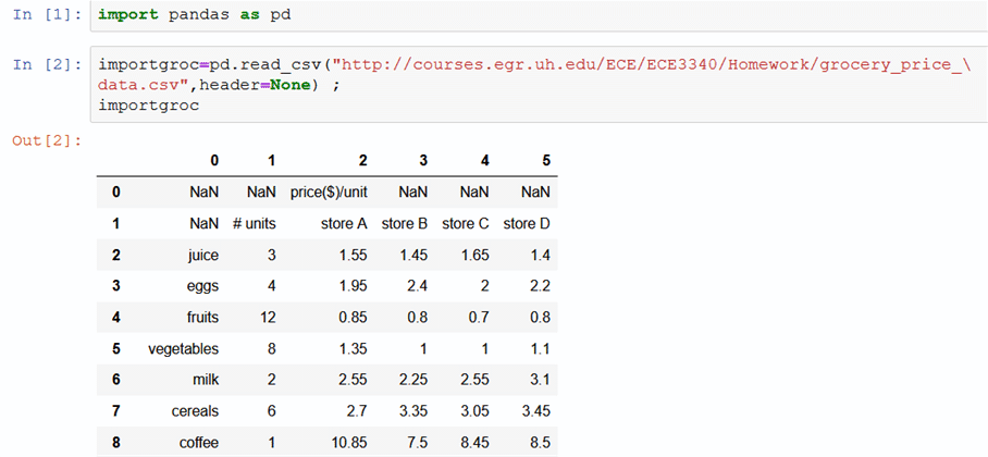
Exercise 2.1
Import the data from .csv file given, obtain the price table and name it something.
Answer
In[4]:=
![]()
Out[4]=

In[5]:=
![]()
Out[5]=

In[13]:=
![]()
Out[13]=
| price($)/unit | |||||
| # units | store A | store B | store C | store D | |
| juice | 3 | 1.55 | 1.45 | 1.65 | 1.4 |
| eggs | 4 | 1.95 | 2.4 | 2 | 2.2 |
| fruits | 12 | 0.85 | 0.8 | 0.7 | 0.8 |
| vegetables | 8 | 1.35 | 1 | 1 | 1.1 |
| milk | 2 | 2.55 | 2.25 | 2.55 | 3.1 |
| cereals | 6 | 2.7 | 3.35 | 3.05 | 3.45 |
| coffee | 1 | 10.85 | 7.5 | 8.45 | 8.5 |
| tea | 2 | 4.2 | 4.15 | 3.75 | 3.95 |
| ice cream | 3 | 7.35 | 6.75 | 6.75 | 4.95 |
| napkins | 5 | 1.1 | 1.2 | 1.2 | 1.25 |
| foils | 2 | 3.5 | 3.75 | 3.6 | 3.75 |
| storage bags | 10 | 0.8 | 0.7 | 0.85 | 0.7 |
| toothpaste | 4 | 1.6 | 1.6 | 1.55 | 1.6 |
| shampoo | 3 | 3.55 | 2.6 | 2.9 | 2.7 |
| detergent | 2 | 9.55 | 9.05 | 8.65 | 7.1 |
![]()
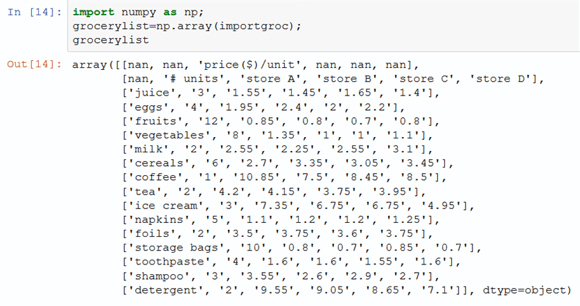
In typical
Jupyter notebook, this is what it looks like
2.2 Referencing elements from a multi-D array
2.2.1 Review: from Tutorial 2
Consider this two dimensional array
In[29]:=

Out[30]=
| 0 | 1 | 2 | 3 | 4 | 5 | 6 | 7 |
| 8 | 9 | 10 | 11 | 12 | 13 | 14 | 15 |
| 16 | 17 | 18 | 19 | 20 | 21 | 22 | 23 |
| 24 | 25 | 26 | 27 | 28 | 29 | 30 | 31 |
| 32 | 33 | 34 | 35 | 36 | 37 | 38 | 39 |
In[31]:=
![]()
Out[31]=
![]()
In[67]:=
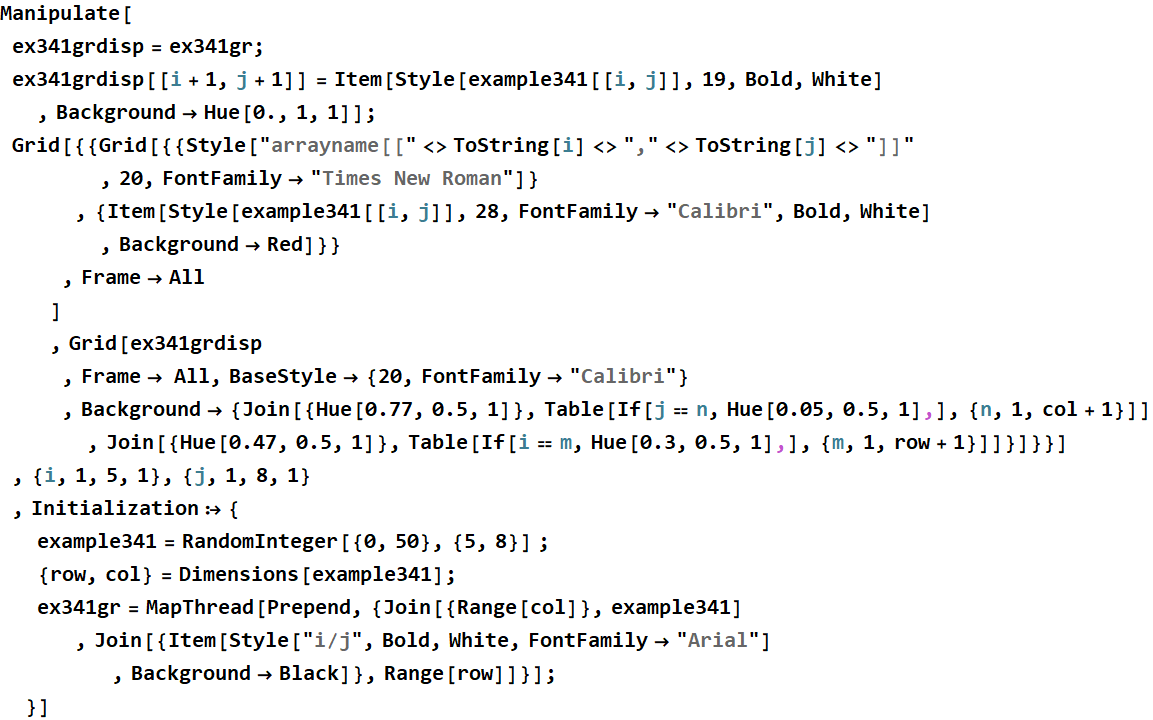
Out[67]=
2.2.2 Sub-array and slice
Consider this:
Out[13]=
| price($)/unit | |||||
| # units | store A | store B | store C | store D | |
| juice | 3 | 1.55 | 1.45 | 1.65 | 1.4 |
| eggs | 4 | 1.95 | 2.4 | 2 | 2.2 |
| fruits | 12 | 0.85 | 0.8 | 0.7 | 0.8 |
| vegetables | 8 | 1.35 | 1 | 1 | 1.1 |
| milk | 2 | 2.55 | 2.25 | 2.55 | 3.1 |
| cereals | 6 | 2.7 | 3.35 | 3.05 | 3.45 |
| coffee | 1 | 10.85 | 7.5 | 8.45 | 8.5 |
| tea | 2 | 4.2 | 4.15 | 3.75 | 3.95 |
| ice cream | 3 | 7.35 | 6.75 | 6.75 | 4.95 |
| napkins | 5 | 1.1 | 1.2 | 1.2 | 1.25 |
| foils | 2 | 3.5 | 3.75 | 3.6 | 3.75 |
| storage bags | 10 | 0.8 | 0.7 | 0.85 | 0.7 |
| toothpaste | 4 | 1.6 | 1.6 | 1.55 | 1.6 |
| shampoo | 3 | 3.55 | 2.6 | 2.9 | 2.7 |
| detergent | 2 | 9.55 | 9.05 | 8.65 | 7.1 |
What if we want a row or a column of the above? Obviously, we can use Table:
In[64]:=
![]()
Out[64]=
![]()
But there is a way to do that with less typing
![]()
Out[65]=
![]()
Exercise 2.2
Define variable itemname and obtain from the table.
Answer
In[68]:=
![]()
Out[68]=

![]()
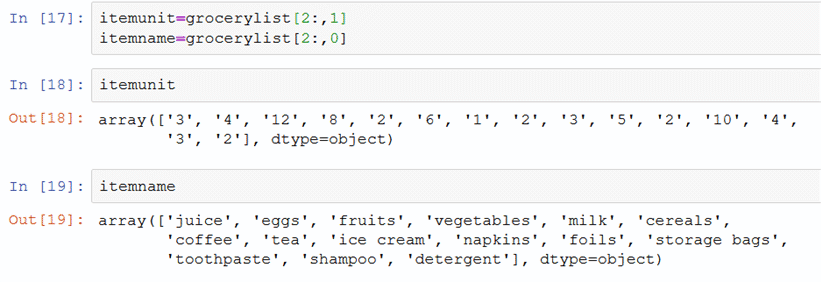
Don�t forget to do conversion from string to float.

For an experienced numpy user:

Exercise 2.3
Define variable storename and obtain from the table.
Answer
In[70]:=
![]()
Out[70]=
![]()
2.3 Matrix and vector dot product
Now, should we obtain the price list of each store? It�s OK to do for 4 stores, but what if you are doing market research for 10,000�s of store in the US? We don�t do price list for each store, we do for all stores.
Out[13]=
| price($)/unit | |||||
| # units | store A | store B | store C | store D | |
| juice | 3 | 1.55 | 1.45 | 1.65 | 1.4 |
| eggs | 4 | 1.95 | 2.4 | 2 | 2.2 |
| fruits | 12 | 0.85 | 0.8 | 0.7 | 0.8 |
| vegetables | 8 | 1.35 | 1 | 1 | 1.1 |
| milk | 2 | 2.55 | 2.25 | 2.55 | 3.1 |
| cereals | 6 | 2.7 | 3.35 | 3.05 | 3.45 |
| coffee | 1 | 10.85 | 7.5 | 8.45 | 8.5 |
| tea | 2 | 4.2 | 4.15 | 3.75 | 3.95 |
| ice cream | 3 | 7.35 | 6.75 | 6.75 | 4.95 |
| napkins | 5 | 1.1 | 1.2 | 1.2 | 1.25 |
| foils | 2 | 3.5 | 3.75 | 3.6 | 3.75 |
| storage bags | 10 | 0.8 | 0.7 | 0.85 | 0.7 |
| toothpaste | 4 | 1.6 | 1.6 | 1.55 | 1.6 |
| shampoo | 3 | 3.55 | 2.6 | 2.9 | 2.7 |
| detergent | 2 | 9.55 | 9.05 | 8.65 | 7.1 |
In[14]:=

Out[15]=
| 1.55 | 1.45 | 1.65 | 1.4 |
| 1.95 | 2.4 | 2 | 2.2 |
| 0.85 | 0.8 | 0.7 | 0.8 |
| 1.35 | 1 | 1 | 1.1 |
| 2.55 | 2.25 | 2.55 | 3.1 |
| 2.7 | 3.35 | 3.05 | 3.45 |
| 10.85 | 7.5 | 8.45 | 8.5 |
| 4.2 | 4.15 | 3.75 | 3.95 |
| 7.35 | 6.75 | 6.75 | 4.95 |
| 1.1 | 1.2 | 1.2 | 1.25 |
| 3.5 | 3.75 | 3.6 | 3.75 |
| 0.8 | 0.7 | 0.85 | 0.7 |
| 1.6 | 1.6 | 1.55 | 1.6 |
| 3.55 | 2.6 | 2.9 | 2.7 |
| 9.55 | 9.05 | 8.65 | 7.1 |
storeprice is now a 2D-array, which can also be
called matrix.
Now, it is too tall, for convenience, we will flip it to the side,
this is called Transpose
In[10]:=

Out[11]=
| 1.55 | 1.95 | 0.85 | 1.35 | 2.55 | 2.7 | 10.85 | 4.2 | 7.35 | 1.1 | 3.5 | 0.8 | 1.6 | 3.55 | 9.55 |
| 1.45 | 2.4 | 0.8 | 1 | 2.25 | 3.35 | 7.5 | 4.15 | 6.75 | 1.2 | 3.75 | 0.7 | 1.6 | 2.6 | 9.05 |
| 1.65 | 2 | 0.7 | 1 | 2.55 | 3.05 | 8.45 | 3.75 | 6.75 | 1.2 | 3.6 | 0.85 | 1.55 | 2.9 | 8.65 |
| 1.4 | 2.2 | 0.8 | 1.1 | 3.1 | 3.45 | 8.5 | 3.95 | 4.95 | 1.25 | 3.75 | 0.7 | 1.6 | 2.7 | 7.1 |
what is the first row of storePrT?
In[75]:=
![]()
Out[75]=
![]()
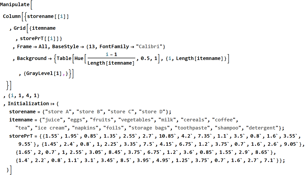
this is the price of store A. Thus:
In[22]:=
Out[22]=
So, it is easy to calculate the cost for each store:
In[84]:=
![]()
Out[84]=
![]()
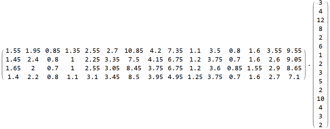
Is it the same as matrix vector product? The answer is yes, and we can simply the code by do this:
In[85]:=
![]()
Out[85]=
![]()
For writing, this is what it usually looks like:
In[86]:=
![]()
Out[86]=
But as we learn in linear algebra, we can also do this:
In[87]:=
![]()
Out[87]=
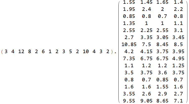
In[88]:=
![]()
Out[88]=
![]()
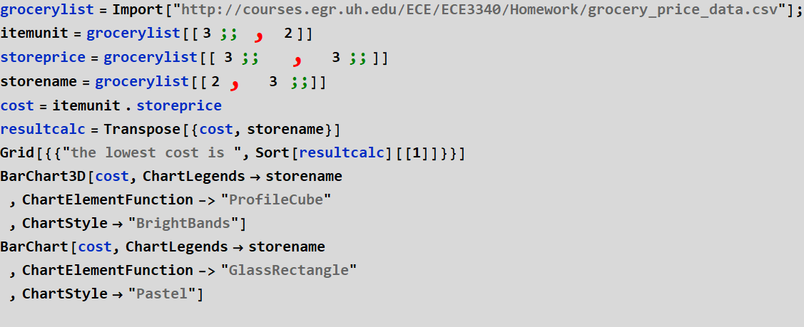
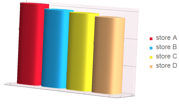
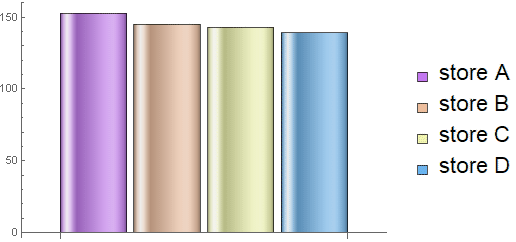
So, the HW 1B problem is quite simple with a few lines:
In[144]:=
Out[145]=
![]()
Out[146]=

Out[147]=
![]()
Out[148]=
![]()
Out[149]=
![]()
Out[150]=
| the lowest cost is | {139.,store D} |
Out[151]=
Out[152]=
2.4 Use App to review matrix dot product
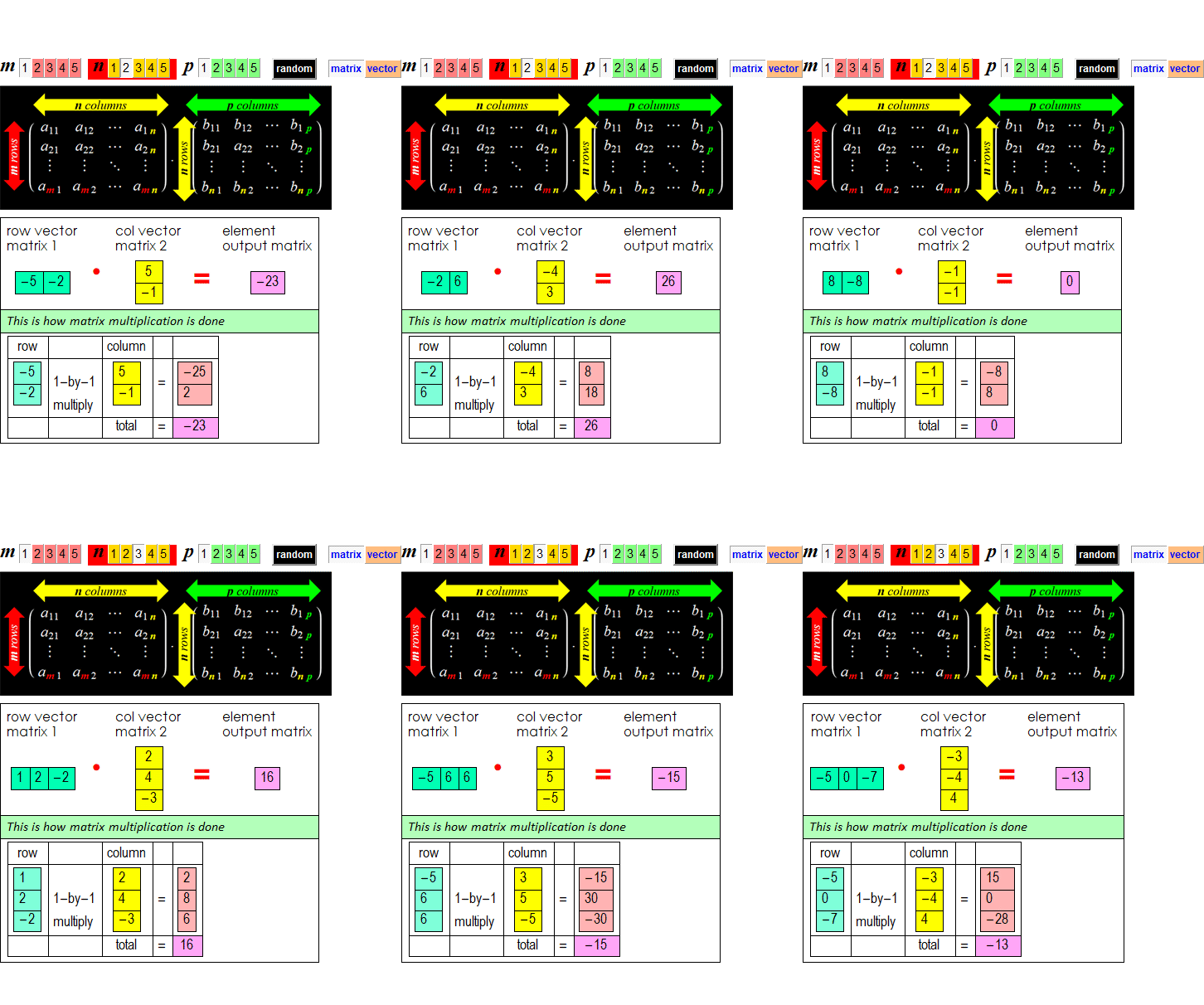
Mathematically, we have two common cases of matrix - vector dot product:
m
� n
matrix n-vector m-vector

and this:
m-vector m
� n
matrix n-vector

Out[1]
Consider the vector dot product:
Next consider the dot product of a
vector (which is 1D matrix) with a matrix:
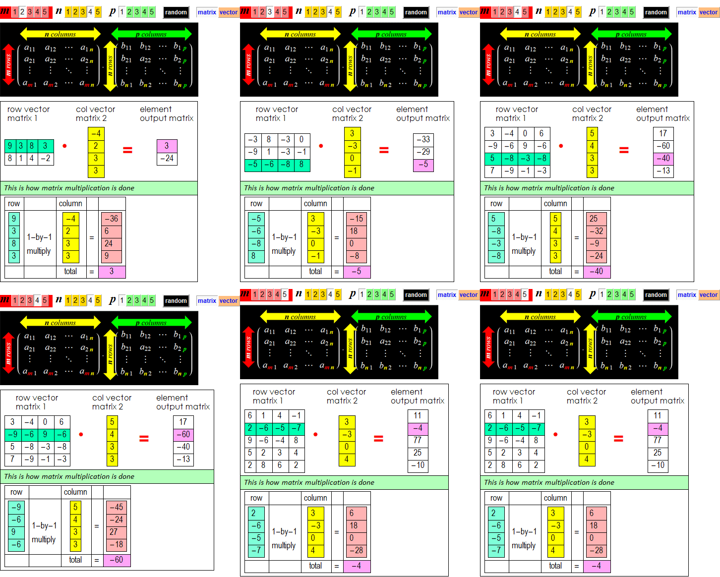
We can also have a "row" vector in
front of a matrix:
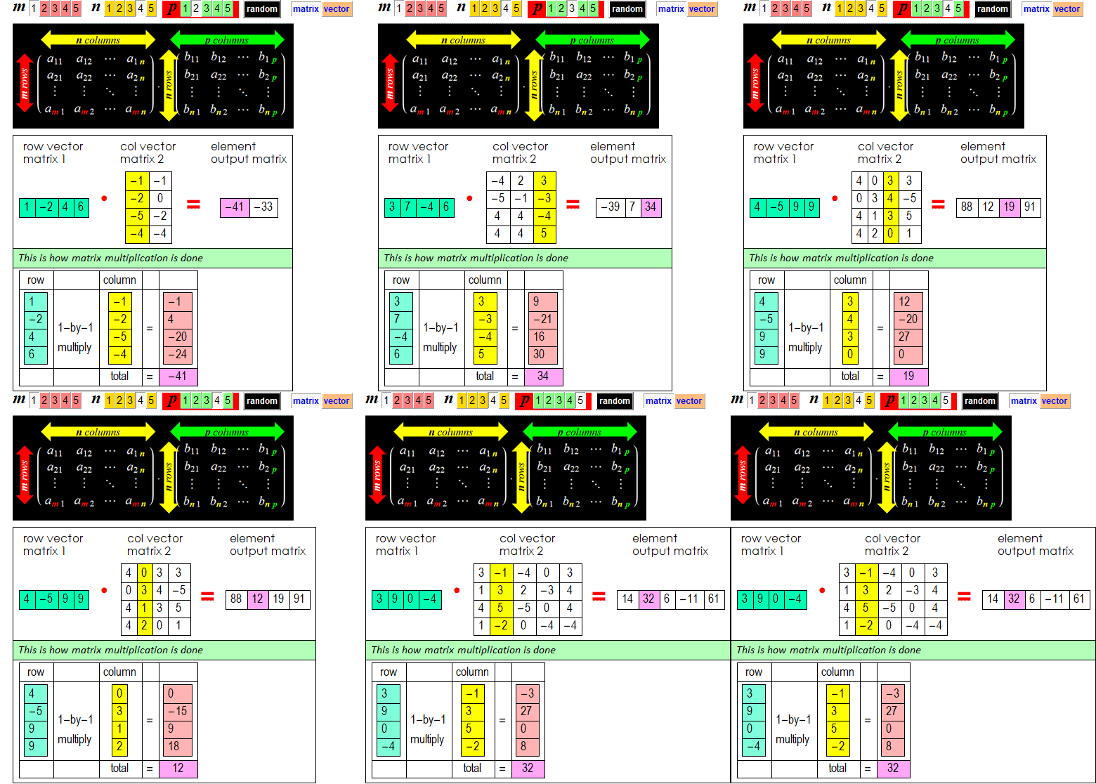
And finally. we have the general
matrix dot product:
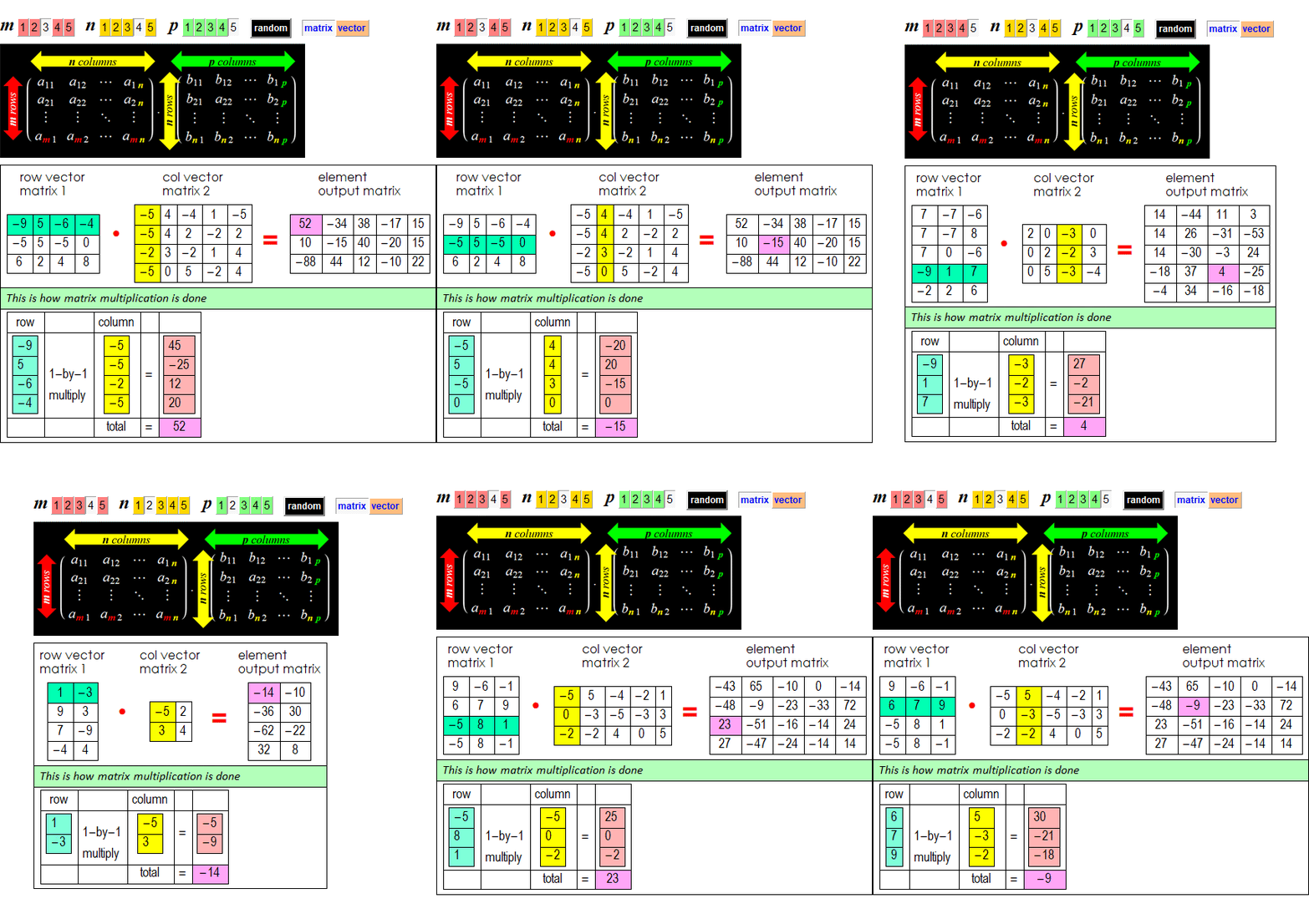
By theorem: ![]()
Hence, we can use transpose whenever convenient.
2.5 Apply learning above with portfolio_data.csv
Exercise 2.4
Write a block code to do similar things as the
example with grocery data file for portfolio_data.csv.
Define variables: dateList, stocksymb, shares, pricedata, with
appropriate values.
(follow instructions in class if needed).
In[95]:=
![]()
Out[95]=
![]()
Answer
We can use exactly the same code for the grocery shopping problem to get answer. Except the variable names are changed or generic (just to avoid confusion)
Also, we use DateListPlot instead of barchart.
In[127]:=
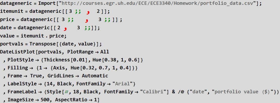
Out[133]=
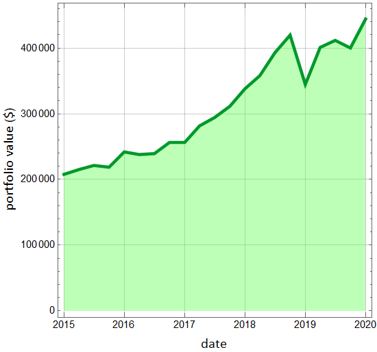
However, if we want to use the same code over and over, we can define a block code.
In[142]:=

Then, we CAN name variables from the generic data according our interest:
In[143]:=

We can find portfolio value at just one time point, say at:
In[145]:=

Out[145]=
![]()
Out[146]=
![]()
End of exercise
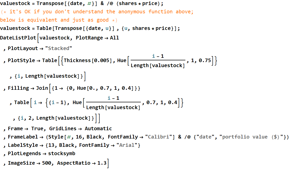
We can do some more for fun:
In[147]:=
Out[149]=
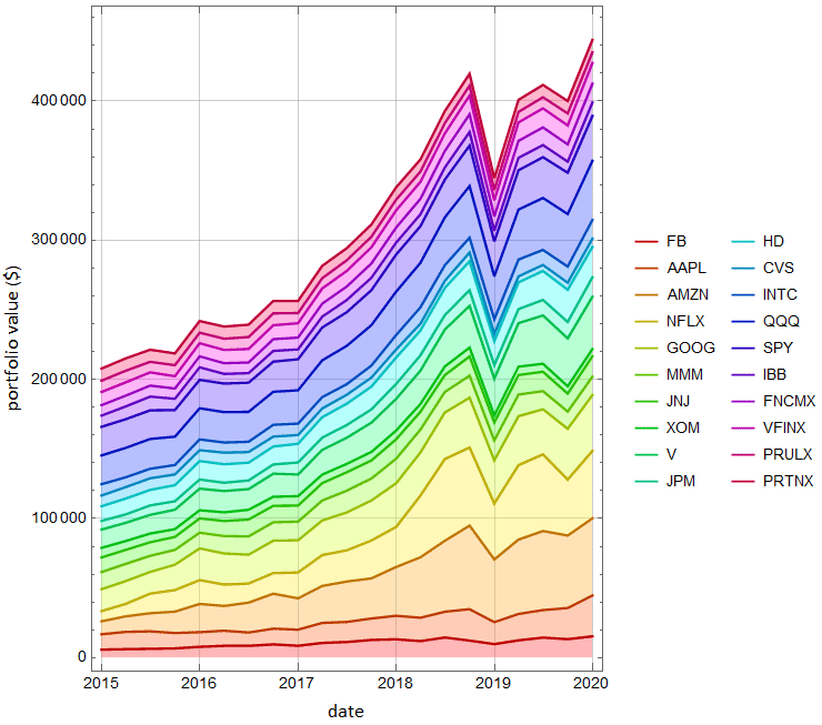
Exercise 2.5
Find the portfolio values (name it value) as a function of time (hint: matrix vector product).
Answer
Should we do this?
In[29]:=
![]()
Out[29]=

The answer is no. There is a much more elegant, mathematically correct, and code-wise efficient way to do, it is matrix vector product:
![]()
Out[103]=

Exercise 2.6
Use DateListPlot to plot portfolio value vs time. You need to pair date (time) with its corresponding portfolio value.
Answer
In[104]:=

Out[104]=
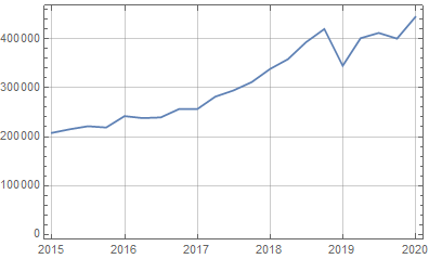
Below shows some styling approach:
In[134]:=

Out[134]=

Mathematically, this is what it looks like:
In[135]:=
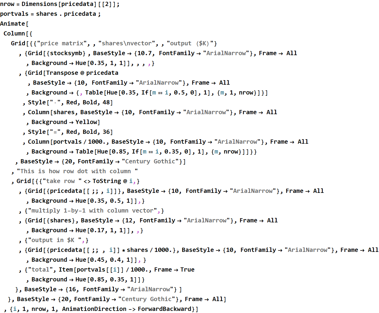
This is known as matrix �dot� vector product. In this case, the vector is a column. Each element of a row of the matrix is multiplied with the same index element of the column, and all are summed together to give an element of the output, which is the value of the portfolio.

For display convenience, we have transposed the price matrix so that each row corresponds to a time point, and the column are the prices of the stocks in green above.
3 General matrix dot product
3.1 Example: hypothetical portfolios
Consider that there are more than 1 client, and the shares are as follow:
In[158]:=

Now, how do we calculate the portfolio for each of them?
In[163]:=

As shown, it is straightforward: the share data are now a matrix of 3 columns for 3 clients (imagine, a brokerage may have millions of clients, and how big their share data matrix is).

This is known as matrix product ot matrix multiplication and matrix-vector dot product is just a special case of matrix dot product.
Review the Matrix Dot Product App again (see 2.4 above):

3.2 Matrix dot product associative property
What if we have this �cascade� problem:
Three bakeries purchase certain quantities of flour and eggs per week as shown below. Given the prices each week, what is the cost of each bakery each week? This is a straight forward matrix multiplication (dot).

Data matrices
Out[92]=
|
|
Exercise 3.1
Three bakeries purchase certain quantities of flour and eggs per week as shown. Given the prices each week, what is the cost of each bakery each week?
Answer
This is a straight forward matrix multiplication
In[93]:=

Out[93]=
|
. |
|
= |
|
In[100]:=

Out[100]=
| weekly costs of the bakeries | ||||||||||||||||||||
|
![]()

Exercise 3.2
But now, we can get more into the details. There are 5 types of cakes, the quantity of flour and eggs for each type is shown below
In[166]:=
![Graphics:PlotLabel /. Options[{RowBox[{RowBox[{cakes, =,
RowBox[{{,
RowBox[{GraphicsBox[TagBox[RasterBox[NumericArray[<33,50,4>,
UnsignedInteger8], {{0, 33}, {50, 0}}, {0, 255}, ColorFunction
-> RGBColor],
BoxForm`ImageTag[System`Convert`CommonDump`ConvertText[Byte,
System`Convert`HTMLDump`htmlsave, HTMLEntities ->
{HTMLBasic}, AltMathOutput -> PlotLabel, WindowSize ->
{2000, Automatic}, MathOutput -> PNG, ConvertClosed ->
False, ConvertReverseClosed -> False, ConvertLinkedNotebooks
-> False, CharacterEncoding -> Automatic,
ConversionStyleEnvironment -> None, ConversionRules ->
Automatic, HeadAttributes -> {}, HeadElements -> {}, CSS
-> Automatic, ConvertLinkedNotebooks -> False, MathOutput
-> GIF, GraphicsOutput -> GIF, Graphics3DOutput ->
Automatic, ManipulateOutput -> CDF, ConvertClosed -> True,
ConvertReverseClosed -> False, FullDocument -> True,
AltMathOutput -> FileName, TableOutput -> {TextForm,
Automatic}, AnimationOutput -> Automatic, FilesDirectory
-> HTMLFiles, LinksDirectory -> HTMLLinks, HTMLEntities
-> {HTML}, AllowBlockMathML -> False, ShowStyles ->
True, DataUri -> False, MathMLOptions ->
{UseUnicodePlane1Characters -> False,
IncludeMarkupAnnotations -> False, Entities -> MathML}],
ColorSpace -> System`Convert`CommonDump`ConvertText[RGB,
System`Convert`HTMLDump`htmlsave, HTMLEntities ->
{HTMLBasic}, AltMathOutput -> PlotLabel, WindowSize ->
{2000, Automatic}, MathOutput -> PNG, ConvertClosed ->
False, ConvertReverseClosed -> False, ConvertLinkedNotebooks
-> False, CharacterEncoding -> Automatic,
ConversionStyleEnvironment -> None, ConversionRules ->
Automatic, HeadAttributes -> {}, HeadElements -> {}, CSS
-> Automatic, ConvertLinkedNotebooks -> False, MathOutput
-> GIF, GraphicsOutput -> GIF, Graphics3DOutput ->
Automatic, ManipulateOutput -> CDF, ConvertClosed -> True,
ConvertReverseClosed -> False, FullDocument -> True,
AltMathOutput -> FileName, TableOutput -> {TextForm,
Automatic}, AnimationOutput -> Automatic, FilesDirectory
-> HTMLFiles, LinksDirectory -> HTMLLinks, HTMLEntities
-> {HTML}, AllowBlockMathML -> False, ShowStyles ->
True, DataUri -> False, MathMLOptions ->
{UseUnicodePlane1Characters -> False,
IncludeMarkupAnnotations -> False, Entities -> MathML}],
Interleaving -> True], Selectable -> False],
DefaultBaseStyle ->
System`Convert`CommonDump`ConvertText[ImageGraphics,
System`Convert`HTMLDump`htmlsave, HTMLEntities ->
{HTMLBasic}, AltMathOutput -> PlotLabel, WindowSize ->
{2000, Automatic}, MathOutput -> PNG, ConvertClosed ->
False, ConvertReverseClosed -> False, ConvertLinkedNotebooks
-> False, CharacterEncoding -> Automatic,
ConversionStyleEnvironment -> None, ConversionRules ->
Automatic, HeadAttributes -> {}, HeadElements -> {}, CSS
-> Automatic, ConvertLinkedNotebooks -> False, MathOutput
-> GIF, GraphicsOutput -> GIF, Graphics3DOutput ->
Automatic, ManipulateOutput -> CDF, ConvertClosed -> True,
ConvertReverseClosed -> False, FullDocument -> True,
AltMathOutput -> FileName, TableOutput -> {TextForm,
Automatic}, AnimationOutput -> Automatic, FilesDirectory
-> HTMLFiles, LinksDirectory -> HTMLLinks, HTMLEntities
-> {HTML}, AllowBlockMathML -> False, ShowStyles ->
True, DataUri -> False, MathMLOptions ->
{UseUnicodePlane1Characters -> False,
IncludeMarkupAnnotations -> False, Entities -> MathML}],
ImageSizeRaw -> {50, 33}, PlotRange -> {{0, 50}, {0,
33}}], ,,
GraphicsBox[TagBox[RasterBox[NumericArray[<75,50,4>,
UnsignedInteger8], {{0, 75}, {50, 0}}, {0, 255}, ColorFunction
-> RGBColor],
BoxForm`ImageTag[System`Convert`CommonDump`ConvertText[Byte,
System`Convert`HTMLDump`htmlsave, HTMLEntities ->
{HTMLBasic}, AltMathOutput -> PlotLabel, WindowSize ->
{2000, Automatic}, MathOutput -> PNG, ConvertClosed ->
False, ConvertReverseClosed -> False, ConvertLinkedNotebooks
-> False, CharacterEncoding -> Automatic,
ConversionStyleEnvironment -> None, ConversionRules ->
Automatic, HeadAttributes -> {}, HeadElements -> {}, CSS
-> Automatic, ConvertLinkedNotebooks -> False, MathOutput
-> GIF, GraphicsOutput -> GIF, Graphics3DOutput ->
Automatic, ManipulateOutput -> CDF, ConvertClosed -> True,
ConvertReverseClosed -> False, FullDocument -> True,
AltMathOutput -> FileName, TableOutput -> {TextForm,
Automatic}, AnimationOutput -> Automatic, FilesDirectory
-> HTMLFiles, LinksDirectory -> HTMLLinks, HTMLEntities
-> {HTML}, AllowBlockMathML -> False, ShowStyles ->
True, DataUri -> False, MathMLOptions ->
{UseUnicodePlane1Characters -> False,
IncludeMarkupAnnotations -> False, Entities -> MathML}],
ColorSpace -> System`Convert`CommonDump`ConvertText[RGB,
System`Convert`HTMLDump`htmlsave, HTMLEntities ->
{HTMLBasic}, AltMathOutput -> PlotLabel, WindowSize ->
{2000, Automatic}, MathOutput -> PNG, ConvertClosed ->
False, ConvertReverseClosed -> False, ConvertLinkedNotebooks
-> False, CharacterEncoding -> Automatic,
ConversionStyleEnvironment -> None, ConversionRules ->
Automatic, HeadAttributes -> {}, HeadElements -> {}, CSS
-> Automatic, ConvertLinkedNotebooks -> False, MathOutput
-> GIF, GraphicsOutput -> GIF, Graphics3DOutput ->
Automatic, ManipulateOutput -> CDF, ConvertClosed -> True,
ConvertReverseClosed -> False, FullDocument -> True,
AltMathOutput -> FileName, TableOutput -> {TextForm,
Automatic}, AnimationOutput -> Automatic, FilesDirectory
-> HTMLFiles, LinksDirectory -> HTMLLinks, HTMLEntities
-> {HTML}, AllowBlockMathML -> False, ShowStyles ->
True, DataUri -> False, MathMLOptions ->
{UseUnicodePlane1Characters -> False,
IncludeMarkupAnnotations -> False, Entities -> MathML}],
Interleaving -> True], Selectable -> False],
DefaultBaseStyle ->
System`Convert`CommonDump`ConvertText[ImageGraphics,
System`Convert`HTMLDump`htmlsave, HTMLEntities ->
{HTMLBasic}, AltMathOutput -> PlotLabel, WindowSize ->
{2000, Automatic}, MathOutput -> PNG, ConvertClosed ->
False, ConvertReverseClosed -> False, ConvertLinkedNotebooks
-> False, CharacterEncoding -> Automatic,
ConversionStyleEnvironment -> None, ConversionRules ->
Automatic, HeadAttributes -> {}, HeadElements -> {}, CSS
-> Automatic, ConvertLinkedNotebooks -> False, MathOutput
-> GIF, GraphicsOutput -> GIF, Graphics3DOutput ->
Automatic, ManipulateOutput -> CDF, ConvertClosed -> True,
ConvertReverseClosed -> False, FullDocument -> True,
AltMathOutput -> FileName, TableOutput -> {TextForm,
Automatic}, AnimationOutput -> Automatic, FilesDirectory
-> HTMLFiles, LinksDirectory -> HTMLLinks, HTMLEntities
-> {HTML}, AllowBlockMathML -> False, ShowStyles ->
True, DataUri -> False, MathMLOptions ->
{UseUnicodePlane1Characters -> False,
IncludeMarkupAnnotations -> False, Entities -> MathML}],
ImageSizeRaw -> {50, 75}, PlotRange -> {{0, 50}, {0,
75}}], ,,
GraphicsBox[TagBox[RasterBox[NumericArray[<45,50,4>,
UnsignedInteger8], {{0, 45}, {50, 0}}, {0, 255}, ColorFunction
-> RGBColor],
BoxForm`ImageTag[System`Convert`CommonDump`ConvertText[Byte,
System`Convert`HTMLDump`htmlsave, HTMLEntities ->
{HTMLBasic}, AltMathOutput -> PlotLabel, WindowSize ->
{2000, Automatic}, MathOutput -> PNG, ConvertClosed ->
False, ConvertReverseClosed -> False, ConvertLinkedNotebooks
-> False, CharacterEncoding -> Automatic,
ConversionStyleEnvironment -> None, ConversionRules ->
Automatic, HeadAttributes -> {}, HeadElements -> {}, CSS
-> Automatic, ConvertLinkedNotebooks -> False, MathOutput
-> GIF, GraphicsOutput -> GIF, Graphics3DOutput ->
Automatic, ManipulateOutput -> CDF, ConvertClosed -> True,
ConvertReverseClosed -> False, FullDocument -> True,
AltMathOutput -> FileName, TableOutput -> {TextForm,
Automatic}, AnimationOutput -> Automatic, FilesDirectory
-> HTMLFiles, LinksDirectory -> HTMLLinks, HTMLEntities
-> {HTML}, AllowBlockMathML -> False, ShowStyles ->
True, DataUri -> False, MathMLOptions ->
{UseUnicodePlane1Characters -> False,
IncludeMarkupAnnotations -> False, Entities -> MathML}],
ColorSpace -> System`Convert`CommonDump`ConvertText[RGB,
System`Convert`HTMLDump`htmlsave, HTMLEntities ->
{HTMLBasic}, AltMathOutput -> PlotLabel, WindowSize ->
{2000, Automatic}, MathOutput -> PNG, ConvertClosed ->
False, ConvertReverseClosed -> False, ConvertLinkedNotebooks
-> False, CharacterEncoding -> Automatic,
ConversionStyleEnvironment -> None, ConversionRules ->
Automatic, HeadAttributes -> {}, HeadElements -> {}, CSS
-> Automatic, ConvertLinkedNotebooks -> False, MathOutput
-> GIF, GraphicsOutput -> GIF, Graphics3DOutput ->
Automatic, ManipulateOutput -> CDF, ConvertClosed -> True,
ConvertReverseClosed -> False, FullDocument -> True,
AltMathOutput -> FileName, TableOutput -> {TextForm,
Automatic}, AnimationOutput -> Automatic, FilesDirectory
-> HTMLFiles, LinksDirectory -> HTMLLinks, HTMLEntities
-> {HTML}, AllowBlockMathML -> False, ShowStyles ->
True, DataUri -> False, MathMLOptions ->
{UseUnicodePlane1Characters -> False,
IncludeMarkupAnnotations -> False, Entities -> MathML}],
Interleaving -> True], Selectable -> False],
DefaultBaseStyle ->
System`Convert`CommonDump`ConvertText[ImageGraphics,
System`Convert`HTMLDump`htmlsave, HTMLEntities ->
{HTMLBasic}, AltMathOutput -> PlotLabel, WindowSize ->
{2000, Automatic}, MathOutput -> PNG, ConvertClosed ->
False, ConvertReverseClosed -> False, ConvertLinkedNotebooks
-> False, CharacterEncoding -> Automatic,
ConversionStyleEnvironment -> None, ConversionRules ->
Automatic, HeadAttributes -> {}, HeadElements -> {}, CSS
-> Automatic, ConvertLinkedNotebooks -> False, MathOutput
-> GIF, GraphicsOutput -> GIF, Graphics3DOutput ->
Automatic, ManipulateOutput -> CDF, ConvertClosed -> True,
ConvertReverseClosed -> False, FullDocument -> True,
AltMathOutput -> FileName, TableOutput -> {TextForm,
Automatic}, AnimationOutput -> Automatic, FilesDirectory
-> HTMLFiles, LinksDirectory -> HTMLLinks, HTMLEntities
-> {HTML}, AllowBlockMathML -> False, ShowStyles ->
True, DataUri -> False, MathMLOptions ->
{UseUnicodePlane1Characters -> False,
IncludeMarkupAnnotations -> False, Entities -> MathML}],
ImageSizeRaw -> {50, 45}, PlotRange -> {{0, 50}, {0,
45}}], ,,
GraphicsBox[TagBox[RasterBox[NumericArray[<38,50,4>,
UnsignedInteger8], {{0, 38}, {50, 0}}, {0, 255}, ColorFunction
-> RGBColor],
BoxForm`ImageTag[System`Convert`CommonDump`ConvertText[Byte,
System`Convert`HTMLDump`htmlsave, HTMLEntities ->
{HTMLBasic}, AltMathOutput -> PlotLabel, WindowSize ->
{2000, Automatic}, MathOutput -> PNG, ConvertClosed ->
False, ConvertReverseClosed -> False, ConvertLinkedNotebooks
-> False, CharacterEncoding -> Automatic,
ConversionStyleEnvironment -> None, ConversionRules ->
Automatic, HeadAttributes -> {}, HeadElements -> {}, CSS
-> Automatic, ConvertLinkedNotebooks -> False, MathOutput
-> GIF, GraphicsOutput -> GIF, Graphics3DOutput ->
Automatic, ManipulateOutput -> CDF, ConvertClosed -> True,
ConvertReverseClosed -> False, FullDocument -> True,
AltMathOutput -> FileName, TableOutput -> {TextForm,
Automatic}, AnimationOutput -> Automatic, FilesDirectory
-> HTMLFiles, LinksDirectory -> HTMLLinks, HTMLEntities
-> {HTML}, AllowBlockMathML -> False, ShowStyles ->
True, DataUri -> False, MathMLOptions ->
{UseUnicodePlane1Characters -> False,
IncludeMarkupAnnotations -> False, Entities -> MathML}],
ColorSpace -> System`Convert`CommonDump`ConvertText[RGB,
System`Convert`HTMLDump`htmlsave, HTMLEntities ->
{HTMLBasic}, AltMathOutput -> PlotLabel, WindowSize ->
{2000, Automatic}, MathOutput -> PNG, ConvertClosed ->
False, ConvertReverseClosed -> False, ConvertLinkedNotebooks
-> False, CharacterEncoding -> Automatic,
ConversionStyleEnvironment -> None, ConversionRules ->
Automatic, HeadAttributes -> {}, HeadElements -> {}, CSS
-> Automatic, ConvertLinkedNotebooks -> False, MathOutput
-> GIF, GraphicsOutput -> GIF, Graphics3DOutput ->
Automatic, ManipulateOutput -> CDF, ConvertClosed -> True,
ConvertReverseClosed -> False, FullDocument -> True,
AltMathOutput -> FileName, TableOutput -> {TextForm,
Automatic}, AnimationOutput -> Automatic, FilesDirectory
-> HTMLFiles, LinksDirectory -> HTMLLinks, HTMLEntities
-> {HTML}, AllowBlockMathML -> False, ShowStyles ->
True, DataUri -> False, MathMLOptions ->
{UseUnicodePlane1Characters -> False,
IncludeMarkupAnnotations -> False, Entities -> MathML}],
Interleaving -> True], Selectable -> False],
DefaultBaseStyle ->
System`Convert`CommonDump`ConvertText[ImageGraphics,
System`Convert`HTMLDump`htmlsave, HTMLEntities ->
{HTMLBasic}, AltMathOutput -> PlotLabel, WindowSize ->
{2000, Automatic}, MathOutput -> PNG, ConvertClosed ->
False, ConvertReverseClosed -> False, ConvertLinkedNotebooks
-> False, CharacterEncoding -> Automatic,
ConversionStyleEnvironment -> None, ConversionRules ->
Automatic, HeadAttributes -> {}, HeadElements -> {}, CSS
-> Automatic, ConvertLinkedNotebooks -> False, MathOutput
-> GIF, GraphicsOutput -> GIF, Graphics3DOutput ->
Automatic, ManipulateOutput -> CDF, ConvertClosed -> True,
ConvertReverseClosed -> False, FullDocument -> True,
AltMathOutput -> FileName, TableOutput -> {TextForm,
Automatic}, AnimationOutput -> Automatic, FilesDirectory
-> HTMLFiles, LinksDirectory -> HTMLLinks, HTMLEntities
-> {HTML}, AllowBlockMathML -> False, ShowStyles ->
True, DataUri -> False, MathMLOptions ->
{UseUnicodePlane1Characters -> False,
IncludeMarkupAnnotations -> False, Entities -> MathML}],
ImageSizeRaw -> {50, 38}, PlotRange -> {{0, 50}, {0,
38}}], ,,
GraphicsBox[TagBox[RasterBox[NumericArray[<75,50,4>,
UnsignedInteger8], {{0, 75}, {50, 0}}, {0, 255}, ColorFunction
-> RGBColor],
BoxForm`ImageTag[System`Convert`CommonDump`ConvertText[Byte,
System`Convert`HTMLDump`htmlsave, HTMLEntities ->
{HTMLBasic}, AltMathOutput -> PlotLabel, WindowSize ->
{2000, Automatic}, MathOutput -> PNG, ConvertClosed ->
False, ConvertReverseClosed -> False, ConvertLinkedNotebooks
-> False, CharacterEncoding -> Automatic,
ConversionStyleEnvironment -> None, ConversionRules ->
Automatic, HeadAttributes -> {}, HeadElements -> {}, CSS
-> Automatic, ConvertLinkedNotebooks -> False, MathOutput
-> GIF, GraphicsOutput -> GIF, Graphics3DOutput ->
Automatic, ManipulateOutput -> CDF, ConvertClosed -> True,
ConvertReverseClosed -> False, FullDocument -> True,
AltMathOutput -> FileName, TableOutput -> {TextForm,
Automatic}, AnimationOutput -> Automatic, FilesDirectory
-> HTMLFiles, LinksDirectory -> HTMLLinks, HTMLEntities
-> {HTML}, AllowBlockMathML -> False, ShowStyles ->
True, DataUri -> False, MathMLOptions ->
{UseUnicodePlane1Characters -> False,
IncludeMarkupAnnotations -> False, Entities -> MathML}],
ColorSpace -> System`Convert`CommonDump`ConvertText[RGB,
System`Convert`HTMLDump`htmlsave, HTMLEntities ->
{HTMLBasic}, AltMathOutput -> PlotLabel, WindowSize ->
{2000, Automatic}, MathOutput -> PNG, ConvertClosed ->
False, ConvertReverseClosed -> False, ConvertLinkedNotebooks
-> False, CharacterEncoding -> Automatic,
ConversionStyleEnvironment -> None, ConversionRules ->
Automatic, HeadAttributes -> {}, HeadElements -> {}, CSS
-> Automatic, ConvertLinkedNotebooks -> False, MathOutput
-> GIF, GraphicsOutput -> GIF, Graphics3DOutput ->
Automatic, ManipulateOutput -> CDF, ConvertClosed -> True,
ConvertReverseClosed -> False, FullDocument -> True,
AltMathOutput -> FileName, TableOutput -> {TextForm,
Automatic}, AnimationOutput -> Automatic, FilesDirectory
-> HTMLFiles, LinksDirectory -> HTMLLinks, HTMLEntities
-> {HTML}, AllowBlockMathML -> False, ShowStyles ->
True, DataUri -> False, MathMLOptions ->
{UseUnicodePlane1Characters -> False,
IncludeMarkupAnnotations -> False, Entities -> MathML}],
Interleaving -> True], Selectable -> False],
DefaultBaseStyle ->
System`Convert`CommonDump`ConvertText[ImageGraphics,
System`Convert`HTMLDump`htmlsave, HTMLEntities ->
{HTMLBasic}, AltMathOutput -> PlotLabel, WindowSize ->
{2000, Automatic}, MathOutput -> PNG, ConvertClosed ->
False, ConvertReverseClosed -> False, ConvertLinkedNotebooks
-> False, CharacterEncoding -> Automatic,
ConversionStyleEnvironment -> None, ConversionRules ->
Automatic, HeadAttributes -> {}, HeadElements -> {}, CSS
-> Automatic, ConvertLinkedNotebooks -> False, MathOutput
-> GIF, GraphicsOutput -> GIF, Graphics3DOutput ->
Automatic, ManipulateOutput -> CDF, ConvertClosed -> True,
ConvertReverseClosed -> False, FullDocument -> True,
AltMathOutput -> FileName, TableOutput -> {TextForm,
Automatic}, AnimationOutput -> Automatic, FilesDirectory
-> HTMLFiles, LinksDirectory -> HTMLLinks, HTMLEntities
-> {HTML}, AllowBlockMathML -> False, ShowStyles ->
True, DataUri -> False, MathMLOptions ->
{UseUnicodePlane1Characters -> False,
IncludeMarkupAnnotations -> False, Entities -> MathML}],
ImageSizeRaw -> {50, 75}, PlotRange -> {{0, 50}, {0,
75}}]}], }}]}], ;}], , ingrmat = {{0., 0.3, 0.1, 0.5, 0.4},
{0.75, 0.25, 0.5, 0.2, 0.6}} ;, , Grid[MapThread[Prepend,
{Join[{cakes}, ingrmat] , {, flour quantity, egg quantity}}],
Frame->All]}]](HTMLFiles/Tutorial_3_answer_116.gif)
Out[168]=
 |
 |
 |
|||
| flour quantity | 0. | 0.3 | 0.1 | 0.5 | 0.4 |
| egg quantity | 0.75 | 0.25 | 0.5 | 0.2 | 0.6 |
And the daily quantities of each cake produced by the bakeries are as follow:
In[169]:=

Out[170]=
| bakery A | bakery B | bakery C | |
| 55 | 70 | 40 | |
| 80 | 50 | 40 |  |
| 30 | 45 | 30 |  |
| 25 | 40 | 30 | |
| 60 | 80 | 50 |  |
What are the daily ingredient demands of the bakeries?
Answer
This is what gives the net four and egg demands of the bakeries each week:
In[171]:=

Out[171]=
| bakery A | bakery B | bakery C | |
| 63.5 | 71.5 | 50. | flour quantity |
| 117.25 | 143.5 | 91. | egg quantity |
This is what we did:
In[172]:=

Out[173]=
| 63.5 | 71.5 | 50. |
| 117.25 | 143.5 | 91. |
Then, we multiply the price matrix to the demand matrix to get the cost matrix for the 3 bakeries:
In[95]:=
![]()
Out[95]=
| 3280.38 | 3906. | 2558.5 |
| 4071.75 | 4837.25 | 3177. |
| 3204.63 | 3797.75 | 2501.5 |
| 3446.5 | 4121.75 | 2686. |
End exercise
![]()

In other words: costmatrix = pricematrix . demandmatrix
costmatrix = pricematrix . (ingredientmatrix
. bakeryproductionmatrix)
4
�
3 4�2 ( 2�5 5�3 )
However, can we do this?
costmatrix = (pricematrix . ingredientmatrix) . bakeryproductionmatrix
because pricematrix .
ingredientmatrix = cakeunitcostmatrix
and the total cost can also be obtained by multiplying cake unit
cost with the cake production matrix. This is the cake unit cost
Exercise 3.3
Find the weekly cost of each type of cake, based on the weekly price of the ingredients and the ingredient requirement of each cake type.
Answer
In[85]:=

Out[85]=
|
|
In[177]:=

Out[178]=
| cost of each cake each week | ||||||||||||||||||||||||||||||
|
End exercise
If we know the weekly ingredient cost of each type of cake, and we know how many cakes of each type each bakery makes daily, then, can we find the net weekly ingredient costs of the bakeries? This is the next exercise
Exercise 3.3
Find the weekly ingredient costs of the bakeries, based on the weekly ingredient cost of each type of cake, and the quantities of cakes of the bakeries.
Answer
We can just multiply this with a # of cakes produced by each bakery per week to get the cost
![]()
In[179]:=

Out[180]=
| 3280.38 | 3906. | 2558.5 |
| 4071.75 | 4837.25 | 3177. |
| 3204.63 | 3797.75 | 2501.5 |
| 3446.5 | 4121.75 | 2686. |
End exercise
Clearly:

In other words, there are more than one way to cut a cake. We can
calculate the total flour and egg demand of each bakery per week,
and multiply the ingredient prices to get the cost
OR
we can multiply the ingredient amount of each cake with the weekly
ingredient price to get the weekly cost of each cake, and multiply
to the production volume of the cakes.
Both give the same result.
Mathematically, what it means is that for 3
matrices A, B, C:
(A . B) . C = A . (B . C)
This is known as associative property. From now on, we don�t have
to use parentheses when multiplying many matrices together.
![]()

In[141]:=

Out[145]=
| A.B | C | (A.B).C | ||
 |
. |  |
= |  |
| A | B.C | A.(B.C) | ||
 |
. |  |
= |  |
Exercise 3.4
Do a
demonstration similar to the above to show the associative
property of dot product. It is OK to copy and paste the
code. But you must choose the range of random integer and the
matrix dimensions according to this:
Range of random integer {-r, r} where r is the 2nd largest digit
of your Student ID, but not smaller than 3. For example 1094724 is
your ID. The second largest digit is 7 (9 is the largest).
For matrix dimensions, we need this: {m, n},{n, p},{p, q}
Let m=3rd largest digit of your ID, but not smaller than 3,
n=Min[8, birth month +2], p=Max[3,Floor[birth date/4.]],
q=Max[2,Ceiling[last digit birth year/2]].
If you cannot calculate, use the App below (but you should
verify to understand and know why the results are what they are).
In[203]:=

Out[203]=
Answer
In[204]:=

Out[208]=
| A.B | C | (A.B).C | ||
 |
. |  |
= |  |
| A | B.C | A.(B.C) | ||
 |
. |  |
= |  |
3.3 Transpose theorem
One more frequently-used property is:
![]()
In[154]:=

Out[157]=
| A | B | A.B | |
 |
 |
 |
 |
 |
 |
 |
Exercise 3.5
Do a demonstration of the transpose theorem like above, but matA and matB are based on your range and dimension from Exercise 3.4.
Answer
In[209]:=

Out[212]=
| A | B | A.B | |
 |
 |
 |
 |
 |
 |
 |
End exercise
![]()

3.4 Serious and common errors
In[9]:=
![]()
Out[9]=
![]()
In[10]:=

Out[11]//MatrixForm=

Shoud we do vt3 . matx3 or matx3 . vt3?
In[12]:=
![]()
![]()
Out[12]=
![]()
Error because we are doing this:

The number of row must match with the number of
column. We should do this instead:

In[13]:=
![]()
Out[13]=
![]()
The rule is simple:
In[14]:=
![]()
Out[14]=
![]()
If we have a vector of length 5, it should be on the left side of the matrix. If length 3, it should be on the right side. The actual orientation, row or column doesn�t matter, because Mathematica knows that if it is on the left, it is automatically row, and column if on the right. Hence:
In[15]:=
![]()
Out[15]=
![]()
But the above is not the worst error, because it tells us if there is an error. This is actually worse:
In[16]:=

Out[17]//MatrixForm=

now
In[18]:=
![]()
Out[18]=
![]()
In[19]:=
![]()
Out[19]=
![]()
The above are totally different, but there is no execution error warning. This type of hidden bug is far more serious. It is up to the programmer to determine which one is correct.
Exercise 3.6
Generate an {m,n} matrix and an{n,p} of your
choice, such that n≠m≠p.
Try to dot {n,p} to {m,n} and observe error. Then, do the dot the
correct order to obtain answer.
Answer
3.5 Inverse matrix and determinant
Consider this problem:

the items purchased are 
Consider that the cost ($) for the above purchase
is: 
What are the prices of apple, orange, and pear? This is the equation:

How do we solve?
In[39]:=

Out[39]=
![]()
The linear algebraic way to do it is to take the
inverse matrix:


By definition:

Hence:


In[40]:=

Out[40]=
![]()
indeed, these are the prices.
![]()

Exercise 3.7
Create 2 equations with 2 unknowns, use inverse matrix to solve it.
Answer
Problem 3.8
Consider this circuit:

Solve for its response.
Find steady-state voltage ![]() for harmonic
for harmonic ![]() and
and ![]() of arbitrary input frequency, amplitude, and relative phase.
of arbitrary input frequency, amplitude, and relative phase.
Answer given
The mesh-current equations of the Laplace-transformed circuit is:

where ![]() is the initial current in
is the initial current in ![]() inductor, and
inductor, and ![]() is the initial voltage of
is the initial voltage of ![]() capacitor.
capacitor.
Define 
We can write the Laplace-transformed mesh current simply:

we can find ![]() although it is rather messy:
although it is rather messy:
In[21]:=

Out[23]//TraditionalForm=

It is much easier to look at with substituted numerical values for the components
In[2]:=

Out[4]//TraditionalForm=

Out[6]//TraditionalForm=

Out[8]//TraditionalForm=
![]()
Out[11]//TraditionalForm=
![]()
Out[12]=
![]()
Out[13]=

The roots indicate the transient responses, which can be overdamped, underdamped, or critically damped.
If we are interested only steady state solutions, we can ignore all the transient terms. Start with:
In[264]:=

Out[267]//TraditionalForm=

Then, because we care only for steady-state
solutions, we can also ignore and make all the initial conditions
such as current ![]() in inductors and voltage
in inductors and voltage ![]() in capacitors to be zero. Then:
in capacitors to be zero. Then:

The mes current vector ![]() is obtained by Inverse-Laplace transforming
is obtained by Inverse-Laplace transforming 
Demo of numerical calculation
Out[28]=
End exercise
Can we take the inverse of this?
In[46]:=

Out[47]//MatrixForm=

In[48]:=
![]()
![]()
Out[48]=
![]()
Exercise 3.9
Generate an non-square {m,n} matrix, denote it A.
Take the inverse of A and see what happens.
Then define a new
matrice: ![]() and
and ![]()
Which one, P or Q has inverse, which one doesn�t, and can you
explain or guess why one does and the other doesn�t?
Answer
End exercise
By its definition, only square matrix can be inversed.
Note, by theorem, if ![]() ,
where I is the identity
matrix, then:
,
where I is the identity
matrix, then:
![]() ,
, ![]() , and
, and ![]()
These theorems simply follow the associative and transpose
properties. For example:
Given A, let ![]() and
and ![]() be such that: A
.
be such that: A
. ![]() = I and
= I and ![]() = I
= I
Then, ![]() . (A .
. (A . ![]() )
=
)
= ![]() . I =
. I = ![]()
By associative: ![]() . A) .
. A) . ![]() =
= ![]()
I . ![]() =
= ![]() or
or ![]() =
= ![]()
One important quantity of a square matrix is determinant. In Mathematica, Det[] gives the determinant of a matrix.
Demo: statistical property (Gaussian -> Laplacian distribution) of det of random matrix
In[85]:=

Out[85]=