ECE3340 - HW 3 - Analysis of a selected work from the class

You must answer in the narrative style and in full sentences (good grammar and prose are a plus). Show your thinking and reasoning in your discussion or explanation. Do not just show a number or a graph as your answer. Your work is treated with respect like any technical/scientific article, where figures, tables are used to support the discussion, not the essence. Hence, your discussion is essential.

Instructor’s comments are in italic and highlighted in light red.
This work earns the highest score of the class, hence it is analyzed to show both the goods and the deficiencies that can be improved.

Many in the class also did excellent work with very high score, however, because of length and file size consideration, there is no way to present compiled works of others, and hence this time, only one can be presented.

1. (65 pts + 10 bonus pts) Voice analysis and synthesis

When we produce a constant vowel sound with a constant pitch, such as the sound “u” in “happy birthday to you..u..u...” or “a a r...” in “twinkle, twinkle little star ... a r...a r..”, the sound signal (air pressure variation) is periodic. This problem is to do an empirical study of this phenomenon: When one tries to sing the same pitch (a musical note) but with different vowel sounds, we human can tell the difference. You can follow step-by-step below, but keep in mind that this is not just a collection of calculation exercises, but a technical report of your research that includes experiments, data analysis, interpretation and discussion. Hence, your thinking and discussion is very important.

Here, vowel sound is defined to be any vibration produced by the vocal chord - essentially, vowels are different modes or resonances of the vocal chord vibration, while the tongue, lips and mouth are held in constant position - and hence, they are not necessarily English language vowels. Latin has other vowels for example (https://en.wikibooks.org/wiki/The_Latin_Language/Pronunciation).

In each section completed below, the data collection, manipulation, and calculations will be conducted first then a paragraph explanation/analysis will be provided at the end. There will also be some comments placed throughout if there is an interesting result or more immediate explanations are needed.

1.1 (10 pts) Experimental data

Record your own vowel sounds at the same pitch or as closely as possible for at least 4 different vowels, and up to six (for extra credits). (just think of singing the same note with different vowels).  Show their waveforms that in your judgment (subjective) are distinctive. Of course, you must present raw data (recordings that one can listen to), and whatever plots or graphs for your discussion of their properties. Please organize and label everything clearly.

1.1.1 Recordings (6 in total):

Six vowel choices were selected to better analyze vowel shapes that we think should have similar wave forms i.e. “eeee” and “oooo”, “ahhh” and “ehhh”, “uhhh” and “ohhh”. I thought it would be interesting to view the subtle differences between waves that sound very similar.

In[2]:=

In[3]:=

In[4]:=

In[1]:=

Out[1]=

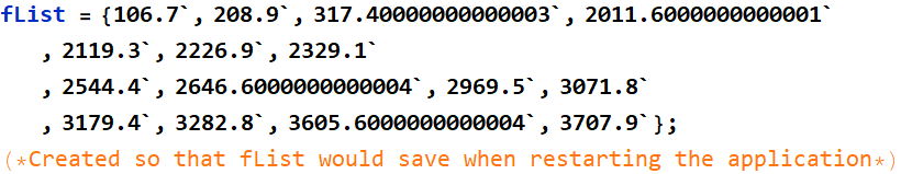
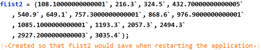
This method of saving the noise was used because once the application was started up again after closing, sound1 was not connected to the audio block. So, while this method may seem strange, it keeps the sound1 variable and the original recording connected on restart.

In[9]:=

In[10]:=

In[3]:=

Out[3]=

In[11]:=

In[12]:=

In[4]:=

Out[4]=

In[17]:=

In[18]:=

In[5]:=

Out[5]=

In[19]:=

In[20]:=

In[6]:=

Out[6]=

In[23]:=

In[24]:=

In[7]:=

Out[7]=

1.1.2 Data extraction and Wave Form Plots:

Data Extraction:

In[8]:=

Instructor’s comments:   If this work can be improved, it would be about handling data: typing 6 lines (or Ctrl+C, Ctrl+V) is OK, but what if one have 10, 20, 100, 10000,...? Below is what one can do:

Out[49]=

Out[51]=

1.1.3 Wave Form Plots (using "ECEgen_APP_PSD_analysis_M12_v0.nb") :

Each set of data points and each sample-rate was imported into the application to acquire what the waveform of each data set looked like to show the distinction between each. A time range of 0.03 seconds was used for each plot because, after some testing, that range seemed to best show the distinctions between the waveforms of each signal.

Instructor’s comments: excellent presentation: perfect clarity, judicious choice and presentation of data.

1. sound1 wave form “ahhh” : (using data1 and srate1)

2. sound2 wave form “eeee” : (using data2 and srate2)

3. sound3 wave form “oooo” : (using data3 and srate3)

This ones pattern is a little harder to see, but after closer inspection, you can tell that the signal is periodic.

4. sound4 wave form “ehhh” : (using data4 and srate4)

5. sound5 wave form “ohhh” : (using data5 and srate5)

6. sound6 wave form “uhhh” : (using data6 and srate6)

1.1.4 Analysis of Wave forms:

Instructor’s comments: Demonstration an understanding of the overall objectives of the HW.

Each plot shows that the signals are periodic so, Fourier’s Theorem will support their recreation. Some signals seem to have much more complex wave forms which might mean that they require more fourier coefficients to recreate accurately like in the case of sound2 and sound4. The signals will have harmonics due to my voice no being able to recreate a perfect cosine wave of tone and it will be interesting to see which signals exhibit which harmonics of the fundamental frequency.

1.2 (15 pts) Data analysis - part 1

Besides the raw sound data and the basic waveform, what other analyses would you perform? (hint: Fourier analysis. Present the power spectral density graphs of the sounds, like a forensic expert, use whichever tools and presentation to make your points, e. g. how the different sounds may have the same pitch, e. g. A4= 880 Hz, but the spectrum of Fourier components are different, etc. Note, no need to produce any specific pitch or real musical note, as long as you feel the pitches are close to each other enough, that’s sufficient).

1.2.1 The PSD [dB] plots of each wave form will be plotted and analyzed below.

A frequency segment of 0 to 4000 [Hz] was used:

Instructor’s comments:  Again, very judicious choice in data presentation. The restriction of frequency range to 4 kHz demonstrates the understanding of “relevance”: Keep relevant data, remove the irrelevant part that only distracts or confuses the reader.

1. sound1 “ahhh” power spectral density graph :

The most apparent frequency was at 1263.04 [Hz]. These very well defined harmonic peaks were taken in a time segment of 0.470227 to 0.911995 [s] of the original signal.

2. sound2 “eeee” power spectral density graph :

The most apparent frequency was at 317.537 [Hz]. These very well defined harmonic peaks were taken in a time segment of 0.487188 to 0.672948 [s] of the original signal.

3. sound3 "oooo" power spectral density graph :

The most apparent frequency was at 430.559 [Hz]. These very well defined harmonic peaks were taken in a time segment of 0.656032 to 0.841791 [s] of the original signal.

The selection to highlight the first and third harmonic of both “oooo” and “eeee” was to highlight the similarities between the wave types. Harmonics are found in all of the presented signals.

4. sound4 “ehhh” power spectral density graph :

The most apparent frequency was at 1625.56 [Hz]. These very well defined harmonic peaks were taken in a time segment of 1.12211 to 1.30787 [s] of the original signal.

5. sound5 “ohhh” power spectral density graph :

The most apparent frequency was at 216.419 [Hz]. These very well defined harmonic peaks were taken in a time segment of 1.3 to 1.62342 [s] of the original signal.

6. sound 6 “uhhh” power spectral density graph :

The most apparent frequency was at 217.423 [Hz]. These very well defined harmonic peaks were taken in a time segment of 1.34517 to 1.6441 [s] of the original signal.

1.2.2 Analysis of PSD plots:

From the collected sound waves and PSD plots, it can be derived that each of the strong harmonic presences are multiples of roughly the same frequency. Each signal’s fundamental frequency is roughly ~105 [Hz] and can be proved with further analysis that can be determined later on. While each signal has a similar fundamental frequency, the difference in vowel shape is emphasized through the varying amplitudes on their harmonics. The more open throat vowel shapes such as “ohhh”, “ahhh”, and “uhhh” seem to have a stronger presence of lower frequencies and the more closed through vowels like “eeee” congregate toward the higher frequencies. Both “ehhh” and “oooo” vowel shapes seem to have an even spread of amplitude in the PSD plot from 0-4000 [Hz]. Each PSD plot does show that they are different signals and hold different attributes in terms of amplitudes and frequencies. The PSD plots are a great tool in distinguishing different waveforms.

Instructor’s comments:    Excellent analysis.

1.3 (20 pts ) Data analysis - part 2 - Fourier theorem and fundamental frequencies.

Demonstrate that the sound wave is truly periodic not by subjective observation (non-scientific and non-rigorous), but with Fourier analysis by measuring many dominant frequencies and showing that they are consistent with Fourier theorem that the dominant frequencies are of the form   where m is an integer (1, 2, 3, ...) and is a fundamental frequency. Find for two of the sounds that you think being most distinctive from each other - your choice. (Hint, for this, you need linear regression and this is a great opportunity to start learning about it a little, and we’ll learn more later. Are the of your various vowels are close to each other? if they do, it means you are a good singer who can consistently produce a pitch - i. e. singing the right note on demand).

1.3.1 Approach: apply Fourier’s theorem (title by instructor)

To better compare the wave forms of each sound, let’s analyze the power spectral density graphs and perform a linear regression of each data set using the same application from the previous section and a helpful provided function provided below. 15 harmonics were chosen from each data set.

findFourier0 Function Definition:

The two sounds that I believe are the most distinctive from each other are the vowel shapes "eeee" and "ohhh" and their linear power spectral density graphs are provided below for analysis :

sound2 “eeee” power spectral density graph (dB) :

sound2 “eeee” power spectral density graph (Linear) :

The most apparent frequency was at 317.537 [Hz].

Collected Harmonics from class provided application:

In[16]:=

In[17]:=

Instructor’s comments:    Again, judicious choice of the order of harmonics that demonstrates an understanding of the Fourier theorem: Not all harmonics are necessary (but OK to select all). The author chooses only the strongest ones, which is sufficient. The objective is to find the fundamental frequency and verify Fourier’s theorem which should be applicable if the data has a truly constant pitch - as opposed to variable pitch such as chirping, or frequency  modulating.

In[18]:=

Out[18]=

sound5 “ohhh” power spectral density graph (dB) :

sound5 “ohhh” power spectral density graph (Linear) :

The most apparent frequency was at 216.419 [Hz].

In[20]:=

In[21]:=

In[22]:=

Out[22]=

1.3.2 Linear regression of the harmonics  (title modified by instructor)

Plot for “eeee” sound:

In[23]:=

Out[23]=

In[24]:=

Out[24]=

Fundamental Frequency of sound2:

In[25]:=

Out[25]=

In[28]:=

Out[28]=

The linear regression seems to fit extremely well and the fundamental frequency is given to be 105.961 [Hz]. To check just how well it fits numerically, I will also perform the “RSquared” function.

In[29]:=

Out[29]=

The”RSquared” output is probably a very long trailing .9999999, so it appears that the regression fits flawlessly, but we can tell it is just almost perfect.

Now lets move on to the linear regression for the "ehhh" sound:

In[26]:=

Out[26]=

In[27]:=

Out[27]=

Fundamental Frequency of sound5:

In[28]:=

Out[28]=

Out[33]=

In[34]:=

Out[34]=

The “RSquared” feature shows that the linear regression is a fantastic fit in both the “eeee” and “ohhh” sounds. There is a discrepancy, however, in the fundamental frequencies of sound2 and sound5.

1.3.3 Analysis:

The sound2 signal exhibits a fundamental frequency, , of 105.961 [Hz] and sound5 exhibits a fundamental frequency of 108.404 [Hz] from the data obtained and analyzed. I would say that if my singing was slightly more consistent that the signals would share almost exactly the same fundamental frequency. As you can see above, each signal is only exhibiting dominant frequencies at multiples of the fundamental frequency, , proving through Fourier’s Theorem that these signals are periodic.

Instructor’s comments:  With a portion of the class presenting data like this:

or
One might wonder if the word “straight” such as in “you should get a very straight line” (repeated ad nauseam in the class) has the same meaning to everyone. This is the reason why R-square is used, which, at the minimum should be 0.999 if not better. This work shows R-square of 1. (which is better than 0.9999995) and 0.999999 for the two vowels.

Below is what an algorithm would yield based on the author’s data.

First, below are the original sounds:the author was capable to generate very constant pitch, better than the class average. As demonstrated in the class, it was suggested that each should take only a snippet of one’s own sound that has a spectrum with sharpest lines. Hence, even if snippet excerpt is not necessary for this author, for the sake of demo, we will take only a snippet of each sound like the rest of the class:

In[27]:=

These are snippets from the originals: audio objects and their waveforns, spectra:

In[28]:=

sndEhhX
  

sndOhhX
  

Now, perform analysis to see what comes out:

Instructor’s comment: Explanation of the print-out results:

Below is the print-out of a coarse iterative search of the harmonics.

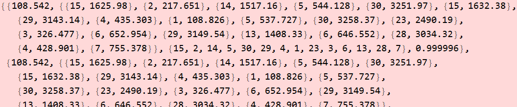
After the coarse search above, it does a fine search, and then linear regression, giving the fundamental harmonics f0 with R-square as shown below.  Notice how little difference between the fundamental harmonics from the coarse search, 108.542 Hz and from the fine search, 108.396 Hz. This indicates the data quality.
The resulting LR fit and residuals are also shown in the graphs.

Finally, using nharmSynth=35: it means 35 Fourier components to reconstruct the sound, it looks quite reasonable:

reconstructed sound	original

Again, coarse search

and fine search. Excellent R-square.

reconstructed sound	original

Instructor’s comment: The results are just as expected. Two things are required:
1- the data itself: it must have constant pitch. If a person’s voice is not steady, just take a snippet where the pitch is steadiest, which shows in the spectrum.
2- get correct and enough Fourier components: this requires good data analysis. Since the software is given to get the Fourier coefficients, the only thing important is to get the good linear regression for accurate fundamental harmonics.

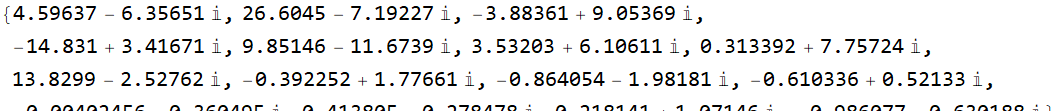
1.4 (5 pts) Data analysis - part 3 - Fourier coefficients

Find the Fourier coefficients that are most closely associated with in 1.3 above.

Instructor’s comment: see the graphs below. they indicate the quality of the data analysis that the author did above.

Finding Fourier Coefficients for sound2 “eeee”:

In[29]:=

In[31]:=

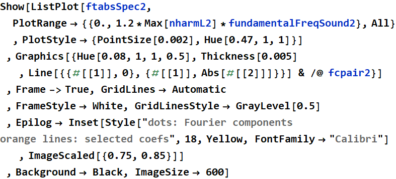
Harmonic Selection with Fourier Components for sound2:

Out[35]=

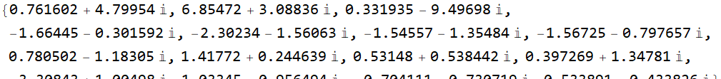
Fourier Coefficients for sound2:

In[32]:=

Out[32]=

In[43]:=

Linear PSD plot with Harmonics Selection for sound2:

Out[45]=

In[36]:=

Decibel PSD plot with Harmonic Selection for sound2:

Out[58]=

Mini Analysis:

The harmonic selection for this vowel shape is more spread out than the harmonic selections of the “ohhh” vowel shape. These plot comparisons help better understand the composition of each vowel shape because after reviewing these graphs, it is clear that since the “eeee” vowel shape is created with a more closed throat, midrange frequency components do not resonate as well.

Instructor’s comments:  Good data analysis produces excellent fit: the graphs of harmonic lines matching with Fourier peaks are proof-in-the-puddings.

Finding the Fourier Coefficients for sound5 “ohhh”:

In[39]:=

In[41]:=

Harmonic Selection with Fourier Components for sound5:

Out[52]=

Fourier Coefficients for sound5:

In[50]:=

Out[50]=

In[42]:=

Linear PSD plot with Harmonics Selection for sound5:

Out[55]=

In[45]:=

Decibel PSD plot with Harmonics Selection for sound5:

Out[61]=

Mini Analysis:

As described in the mini analysis of the “eeee” PSD plots, plotting both the dB and the linear PSD plots together help bring out the characteristics of the vowel shapes. The “ohhh” vowel shape has a very open throat sound and thus contrasts with the “eeee” sound strongly in the fact that more mid range frequencies are not only present but a large source of sound5’s composition.

Analysis:

The cleanest representation of the Fourier’s theorem with coefficients I believe is shown in the “ohhh”/sound5 PSD plot due to how accurate and precise each frequency is represented on the linear plot with little noise and how spread out the fourier coefficients are. In the PSD plot for the “eeee” sound2, the fourier coefficients seem too clumped together and placed in some questionable areas. However, the “eeee” PSD plot is still a good example, just not as clean as the “ohhh” PSD plot. It is a good comparison to see the strong frequencies shown in the dB vs linear PSD plots because the dB PSD plot shows almost all of the components of the signal while the linear PSD plot shows clearly which frequencies are the most impactual.

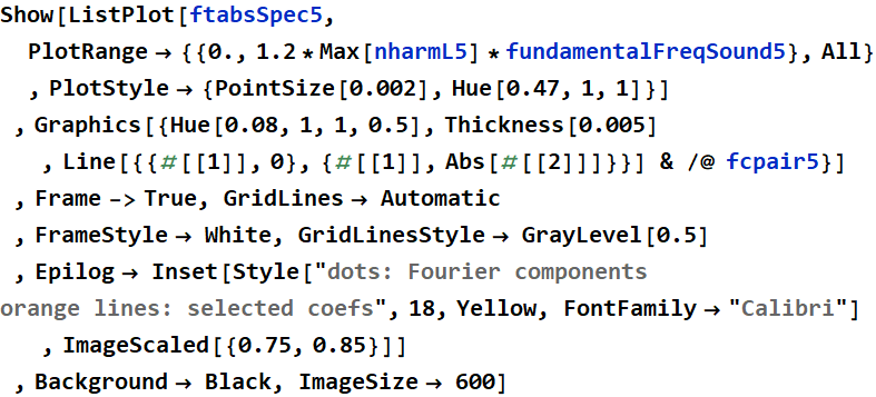
1.5 (15 pts) Fourier-approximation reconstruction

The signals you generated above may have 10 of thousands of Fourier coefficients; all are needed to reconstruct the original waveform exactly. Can we approximate each sound with just ~10 - 20 components, i. e. <0.01% of the Fourier components? Of course it is only an approximation, but the objective of this calculation is to investigate whether the two vowels you choose in 1.3, say, let’s call them and , are distinctive to human hearing (your judgement) based on a very small fraction of their Fourier components.

In other words, and sound very different (according to you). If we partially reconstruct or approximate the two sounds with Fourier synthesis based on only a handful of their dominant Fourier components, would that be sufficient to hear them as being distinctive? Of course, this is subjective but can be considered as a physiological/psychological experiment on human auditory response, and hence this self-reporting subjectivity is a part of the work.

Answer:

Instructor’s comments:  Unfortunately, this is the only part that the author has a minor deficiency: the author uses 15 harmonics to start, and reaches the conclusion that 15 harmonics might not be enough. If 15 was not enough, the logical thing to do is to use more and more until one can see what happens. The results above and duplicated below show 35 Fourier components.

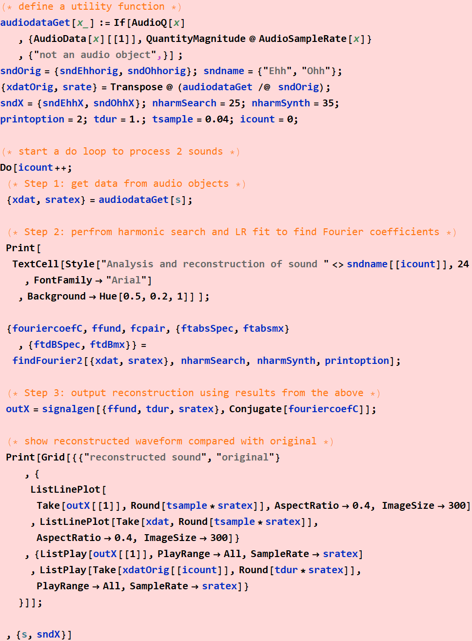
We will utilize the signal generation code provided to analyze the amount of fourier coefficients necessary to recreate the original vowel shapes to an acceptable degree.

In[48]:=

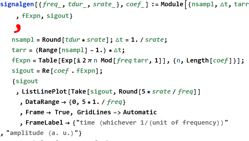
In the code segment below, I opted to use the negative conjugate of the wave since the audio was the same with either positive or negative due to the sound relying on magnitude and frequency and it was better to compare to the original signal because it looked more similar to the wave forms in both cases of sounds “ohhh” and “eeee”.

In[49]:=

In[53]:=

Out[53]=

Generated “eeee” waveform plot:

In[97]:=

Out[97]=

In[54]:=

In[58]:=

Out[58]=

Generated "ohhh" waveform plot :

In[104]:=

Out[104]=

Vowel Comparison:

Audio:

    Synthesized vs. Original:

        sound2/”eeee”:

In[108]:=

Out[108]=

Out[109]=

        sound5/"ohhh" :

In[114]:=

Out[114]=

Out[115]=

Graphical:

    sound2 / "eeee" :

    sound5 / "ohhh" :

Analysis :

    Audio Analysis:

After obtaining the synthesized signal of each vowel, I have deduced that the fourier theorem holds quite well for recreating periodic signals; however, 15 coefficients is not enough to recreated the signal to its original stature by any means. Both of the synthesized signals sound very close to their original signal but still sound more synthetic than intended. I believe that both the sound5 or “ohhh” vowel and the “eeee” vowel shape turned out well in terms of sound replication from their original waves.

    Graphical Analysis:

In terms of the plot comparison of the waveforms, the “ohhh” synthetic plot represents the original wave form much more closely than that of the “eeee” sound. This could be due to the fact that the “eeee” wave may have had a more complex wave form and that requires more fourier coefficients to replicate or maybe the recording itself may not be as high of quality as the “ohhh” recording. Nevertheless, both recordings were able to be successfully replicated to a reasonable degree proving not only that the signals are periodic but also that Fourier’s theorem, yet again, is valid.

Instructor’s comments:  If the author had changed a single parameter in function findFourier0  to make ~30 to 35 Fourier components, the results below would have been obtained and it would make a rare perfect HW.

reconstructed sound	original

reconstructed sound	original

Instructor’s comments:  Although the author obviously has vocal capability to produce a constant pit over a long duration, that is NOT the basis for this excellent HW. It is shown above that all one needs is just a snippet of sound of a fraction of a second, which, everyone in the class is capable of, to get a reconstructed sound like this.

1.6 (10 pts) Fun bonus

After the hard work above, you can use the Fourier components you find to synthesize some music. Produce a tune with more than a few notes but playtime no more than 10 secs with the two sets of coefficients. Do they sound like two different musical instruments?

Code:

Instructor’s comments:  Seems the author had fun, which is exactly the intention of this bonus.

In[75]:=

First made with sound2 “eeee”:

In[88]:=

In[92]:=

In[96]:=

Out[97]=

Now made with “ohhh”/sound5:

In[66]:=

In[70]:=

In[74]:=

In[78]:=

Out[79]=

Song created with “eeee” vowel shape:

Song created with “ohhh” vowel shape:

Analysis:

The song made with the “ohhh” vowel shape sounds more like a woodwind instrument, maybe a tenor saxophone and the song made with the “eeee” vowel shape sounds like an electric keyboard. I like this exercise because it better highlights the differences between the two vowel shapes than just playing a singular note.

2. (35 pts) Signal and noise

2.1 (10 pts) Generate a sound, and with added noise

You can re-use any of the sound you generated in Problem 1. If you don’t do Problem 1, then generate a sound per the instruction of 1.1. The duration of your recording should be ~1 sec if using 44.1 kHz sampling rate, or 2 sec if using 22.05 kHz (so that the data length is roughly the same).
1- Find the root-mean-square of your signal, call it .
2- Generate a Gaussian noise of the same length with standard of deviation σ= 5 *
3- Add them together
4- Play all three: recorded sound, noise by itself, and signal+noise
Discuss (even if you feel you are stating the obvious).

1. Find the RMS of signal of synthesized “ohhh” vowel shape:
    a. Synthesize signal with a duration of 1 second:

Instructor’s comments:  exactly follow the instruction.Very clear each step.

In[98]:=

    b. Take the RMS:

In[102]:=

Out[102]=

2. Generate a Gaussian noise for 1 second with a standard deviation of σ= 5 * (RMS signal)

In[32]:=

In[67]:=

Out[67]=

3. Add the original signal to the Gaussian white noise:

In[34]:=

4. Play all three signals (original, noise, combined):

In[38]:=

Out[38]=

Out[39]=

Out[40]=

Discussion:

Above I have calculated the RMS value of my synthesized signal OneSecSignalOhhh. Using this value, I was able to generate a noise with σ= 5 * (RMS signal). Finally, I played all three signals, (original, noise, and combined), to then find that in the combined signal, totalSignal, that the original signal is very faint and that the noise over powers it. This is most likely due to generating a noise with 5 times the RMS value of the original signal.

2.2 (20 pts) Spectral analysis and signal-to-noise ratio

Do spectral analysis of all three for the entire duration of the sound (~ 1 sec). Then, do spectral analysis of signal +noise for the following: ~1/16 of duration (any segment you wish within the signal), 1/8, 1/4, 1/2. Discuss what you observe and plot what you think as signal to noise ratio vs sample duration on log-log scale. (Just state your fact-based observation, save your interpretation for Q. 3 below).

Instructor’s comments:  This is excellent in terms not only presentation, but a broad understanding of the objective of this excercise. The clincher is the LogLog plot of the signal-to-noise ratio below. Excellent work!

1. PSD plot for OneSecSignalOhhh:

15 distinct points are shown in representing the harmonics of the generated signal, lets see how many will still be distinguishable after the noise is added.

2. PSD plot for gNoise:

This plot of the noise generated does not reach the same decibel levels that the original signal does, so maybe it will still be possible to see most of the harmonic peaks in the combined signals.

3. PSD plot for totalSignal:

Only about 8 peak harmonics of the original frequency components are discernable with the noise added in. But the strongest frequency component still remains to be 217 [Hz].

Instructor’s comments:  It is important to observe how distinctive the signal (i. e. its Fourier components) compared to the noise. The author understand exactly what we are looking for.

4. To obtain a log plot of the frequency to noise ratio, I am going to gather a fourier component from a part of the original signal present in the combined signal PSD and take its ratio with the magnitude of the mean of the noise and plot over a 1/16, 1/8, 1/4, 1/2 log-log plot.

In[72]:=

Out[72]=

Using the above statement, I have created an average of the noise signal to create a ratio of original signal to noise signal.

I clipped my original audio to a 16th of its original length to get the amplitude of its strongest frequency to create a original signal to noise ratio.

In[81]:=

Out[81]=

I found this to be the maximum amplitude in the 1/16 data segment in order to complete the ratio. The maximum amplitude was found at a frequency of 223.858 [Hz];

In[82]:=

Out[82]=

The same process executed above is completed for the rest of the time segments below:

In[80]:=

Out[80]=

I found this to be the maximum amplitude in the 1/8 data segment in order to complete the ratio. The maximum amplitude was found at a frequency of 215.941 [Hz];

In[83]:=

Out[83]=

In[84]:=

Out[84]=

I found this to be the maximum amplitude in the 1/4 data segment in order to complete the ratio. The maximum amplitude was found at a frequency of 219.96 [Hz];

In[85]:=

Out[85]=

In[87]:=

Out[87]=

I found this to be the maximum amplitude in the 1/2 data segment in order to complete the ratio. The maximum amplitude was found at a frequency of 215.99 [Hz];

In[88]:=

Out[88]=

LogLogPlot of signal to noise ratio:

Instructor’s comments: this chart is the result that this problem is designed for.

In[90]:=

In[97]:=

Out[97]=

Analysis:

My method to obtain the loglog plot may be somewhat odd, but I believe that it makes sense. I took the FFT of the noise signal and took the average of all of the peaks of the noise signal in order to get an average value of the noise. Then I took the FFT of the original signal at each time segment 1/16, 1/8, etc, found the peak harmonic each time, and found that the peak magnitude at the same frequency was increasing. Using the magnitude of the peak frequency at each time segment and creating a ratio with the noise average showed an increase as the time segment of the recording was increased. As the time segment for the total signal increased, the ratio of original signal to noise increased and on a loglog plot appears linear.

Instructor’s comments: The Log Log Plot is not odd at all. It is exactly stated in the question: “Discuss what you observe and plot what you think as signal to noise ratio vs sample duration on log-log scale”. If something is linear on Log-Log scale, it means a power law: where a is the slope of the line on log-log. This slope is 1 as expected.

2.3 (5 pts) Broader interpretation

What would be your interpretation of the results in 2.2?

Instructor’s comments: The intuitive interpretation by the author, as opposed to a formal analysis based on both DFT and Parseval’s theorem is the intended objective. This answer nails it.

The time segment selected, (1/16, 1/8, 1/4, 1/2), of the original signal would increase not only the power of the strongest frequency, shown in the PSD plot, but also the magnitude of its fourier component. A possible reason why the fourier component of the harmonics of the original signal would become stronger as the time segment became larger is due to the FFT having more data points to analyze and to better pin point the actual harmonic of the signal. More points creates better resolution, so the signal is better defined and perhaps stronger. The increase in the signal’s frequency components and amplitudes also seems to have a logarithmic increase and so it was best to plot the ratio to time segment on a log log plot.

3. (20 pts) Bonus extra - musical instruments

Why do different musical instruments playing the same note sound differently? Here, we are not talking about the envelope or modulation of the sound. For example, both piano and harpsichord involve a hammer hitting a string, which results in an exponential decay envelope as shown below, but still sounds different (it wouldn’t be called pianissimo if there were no difference, right?).

In[1]:=

Out[2]=

Likewise, strings, woodwinds, or brasses all sound differently even if played with a similar envelope. (If all instruments sounded the same, there wouldn’t be such a thing as an orchestra, would it?). This is a bonus problem, and hence, it is totally free form, but don’t write more than three pages including figures. No need to overkill, just comparing and discussing a few instruments are sufficient. Do it only if you really enjoy or passionate about the topic, don’t do it just for bonus. Just a point for your amusement: If a violin plays the same note two times, it would sound roughly the same; but a human can sing the same note with different vowels.

Discussion:

Instructor’s comments: Very well research. Only one weakness: no spectral analysis of the two types of guitar. But it’s quite good.

The reason that instruments sound different, excluding the fact of different envelopes, is that different harmonics strengths are highlighted in different instruments and different vowel shapes. This idea was exemplified throughout this entire homework because both of my generated signals have the same envelope, no envelope, and yet they sound different because they have different strengths at different harmonics. A default envelope for any instrument is provided below and is typical of instruments like a trumpet or other wind instruments.


Let’s take a look at different instruments with similar envelopes:

Ex: tuning fork, piano, xylophone.

Sources for Above Audio:

https : // amath.colorado.edu/pub/matlab/music/wav/tuning_fork _A4.wav
https://freesound.org/people/DANMITCH3LL/sounds/232004/
https://samplefocus.com/tag/piano-note

These all have the same type of envelope, maybe with different rates of decay but still similar, as described above but the difference is in how many harmonic components are expressed/heard because of how the instrument was constructed. Each of the above instruments are struck once and decay in a way plotted at the beginning of this question. There are so many different components that go into how an instrument sounds. Take an acoustic guitar and an electric guitar for example. Both instruments are guitars, but the tone in each can sound vastly different. An acoustic guitar focuses on acoustics in its harmonic construction of its unique noise, but the electrical guitar focuses more on the electrical pickups for its tone and the signal can be altered through an amplifier as well depending on whether or not the amplifier is a tube amplifier or a solid state amplifier. Some harmonics might flourish better in a physical environment such as how the acoustic guitar is constructed, but some harmonics may be near impossible to hear without an electrical focused arrangement like in the case of the electrical guitar. While some may argue that the amplifier may count as modulating the signal and that is why the instruments sound different - take away the amplifier. Without any amplification, both guitars, acoustic and electric, can play the same string, same fret, same note and still sound different because different harmonics are exemplified in the physical construction of each instrument. The acoustic guitar will typically have a fuller bodied sound because the gauge of string is larger on acoustic guitars and because the body is designed to resonate strongly. An electric guitar is going to tend to have a more shrill tone because the string gauge is smaller than that of an acoustic and because most electric guitars do not have a hollowed out section for resonance. Images and recordings are provided below for examples and for fun:

In[106]:=

In[108]:=