An example of a free-form problem
Han Le - Copyrighted
0. Consideration - following the guideline
1- Find an electrical engineering problem that should be solved with materials covered in this course Numerical Methods. Think of the follow:
• What EE courses have you taken?
• What were some problems that you encountered in those courses?
• What new, creative “twists” can you introduce into one of those problems?
• Do you think you can solve that problem (with a new twist preferably), by applying what you learned in this class?
outcome: an op-amp circuit
A problem from a course in circuit: how to make a square wave oscillator with op-amp.
Consider the op-amp circuit below:
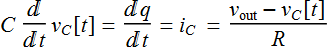
We want to solve for ![]()
According to op-amp theory: ![]()
where ![]() is the open-loop gain. But
is the open-loop gain. But ![]() is extremely large, hence, unless
is extremely large, hence, unless
![]()
we have: 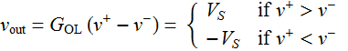
We can find ![]() as follow.
as follow.
We see that:  where we define:
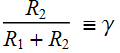
![]()
![]() ;
; 

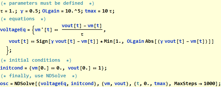
Now, we are ready to use NDSolve to solve a nonlinear system of differential equations.
1. Numerical Method with NDSolve
Setup
1. Write code for equations
vp, vm, and vout are ![]() ,
, ![]() , and
, and ![]() . Let:
. Let: 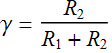
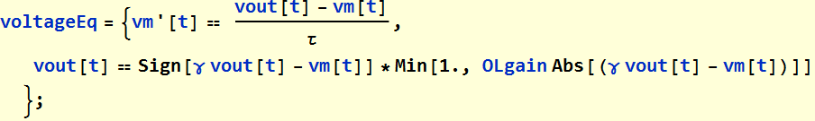
the equations are:

We notice that the relationship 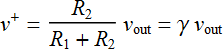 is just too simple to make it an equation. Hence, we eliminate
 ![]() and substitute it with
and substitute it with ![]() to have only 2 equations: (this save a little computation time)
to have only 2 equations: (this save a little computation time)
2. Write code for inititial conditions
We need initial conditions:
Let just set vm[t=0]=0. At that point, vp can be positive or negative depending on vout. Let’s assume vout=1.
![]()
Let’s choose:
3. Define parameters
![]()
4. Put all together according to correct order
Now we use NDSolve
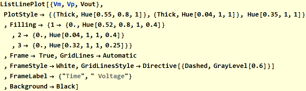
5. Plot to look at solutions
We will plot ![]() ,
, ![]() which is
which is ![]() and
and ![]()
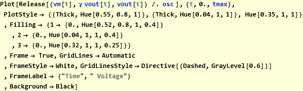
It works. It shows that the circuit is indeed a bistability system with output that flipflops between 2 states. This is just an illustration of the very high-gain behavior of an open-loop op-amp: the voltage output is saturate at either max positive or max negative ![]() and hence generates a square wave.
and hence generates a square wave.
What we do here is to demonstrate it with brute-force numerical differential equation solution rather than circuit analysis. In fact, if we didn’t do circuit analysis, this method helps us gain insight so that we can go back to do circuit analysis and understand what happens.
Manipulatable parameters
As a final step, we now put the whole thing in a dynamic loop so that we can vary the circuit parameters τ and γ.
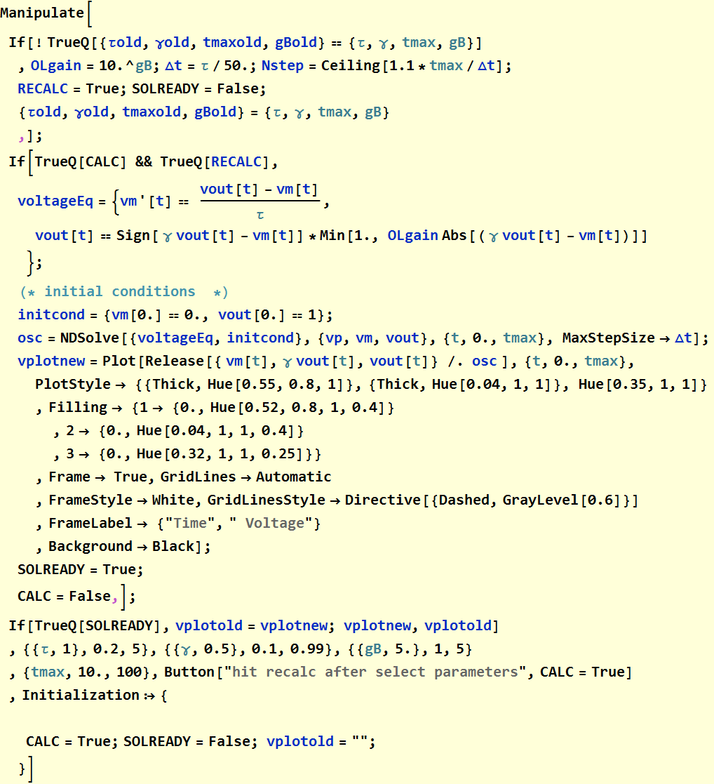
Put into an app structure
2. Time-step (Finite-difference) simulation of op amp square-wave generator
Discussion
We see the above NDSolve does the job, but it is slow as expected. We can have a different appraoch, based on the insight we gain above that is faster. In this approach, we solve the problem as time-domain difference equation: we make the step in time and update the discrete values of the voltages at the sampling time point.
But we can go even further: we can solve the simple and straight forward equation:
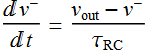
whenever ![]() is not at a transition point, because it is always a constant otherwise, either
is not at a transition point, because it is always a constant otherwise, either ![]() or
or ![]() .
.
Thus, treating ![]() as a constant:
as a constant:
![]()
![]()
![]() is just a constant to be determined by initial condition. The tricky thing here, however is that we should choose the initial condition to be the starting point of a cycle, which is where
is just a constant to be determined by initial condition. The tricky thing here, however is that we should choose the initial condition to be the starting point of a cycle, which is where ![]() just flips and starts its constant value for 1/2 a cycle.
just flips and starts its constant value for 1/2 a cycle.
That point is where ![]() . Thus, we can choose that as t=0:
. Thus, we can choose that as t=0:![]()
Now we can write the code
Code development
Equation for time step
Test with a Do loop
Plot the result:
It works as expected.
Manipulate loop for control of parameters
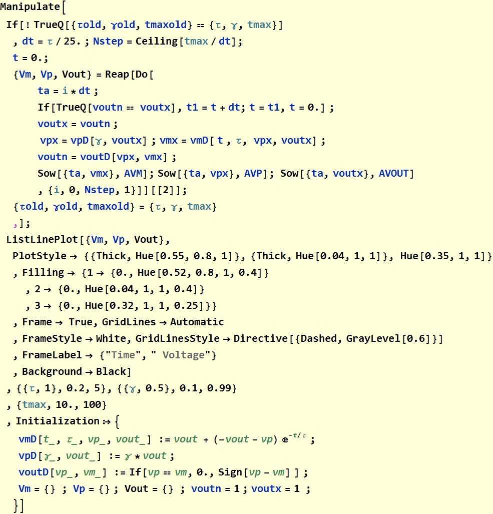
Put into an app structure
3. Op amp square-wave sound generator
We can put the waveform into an amplifier and speaker to listen to it.