HW 12 - Answer

ECE 5368/6358               han q le - copyrighted
Use solely for students registered for UH ECE 6358/5368 during courses - DO NOT distributed (copyrighted materials)

Overview

The objective of this HW is for you to learn and apply the numerical Fourier method (discrete Fourier transform) to solve optics problem.
The math of Fourier transform is absolutely essential for the understanding of various optical phenomena. It can appear difficult at first if one has not had much experiences in studying and using Fourier transform.
This HW is designed to help you learn it via the computation method. The computer codes are given to make it easy even if you didn’t have much experience. The objective is for you to at least understand the idea and the procedure how to do it.
Read and follow instructions closely and you will find it easy. There are two essential external APPs (not included in this file) that are required to do the work. Download and test them. Don’t wait until last minutes.

Important: DELETE the entire hint/help section in each question or wherever you find it.

The hint/help is for you to use. Cut and paste it in a separate scratch notebook (the whole help section, not just the section header). Copy only the results into your answer along with discussion/explanation. Do not leave the hint in.

1. (50 pts) Pulse spectrum

If we have a pure monochromatic light source with constant power
                                               ,
we can use a beam chopper, or an amplitude modulator to make pulses like the APP below.

1.1 (35 pts) Δt Δν relationship

Select a pulse shape according to your student ID last digit as follow:

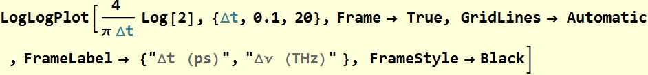
Vary the full-width half max (FWHM) pulse E amplitude duration Δt for 5 values between 1 to 10 ps (any value in that range) and measure the FWHM bandwidth Δν of the Fourier spectrum. Plot relationship of Δν vs. Δt on log-log scale. What do you observe of their product Δt Δν? Discuss.
Note: you don’t have to show all your pulses and their corresponding spectra. You only have to show at least one pulse and its spectrum and the value of  Δt and Δν that you obtain (this is to verify that you know how to read full-width half max).

Answer

You should get a straight line showing inverse relationship of Δt and Δν on a log-log plot.
Below is the code showing how to obtain FWHM:

How to obtain full width half max

The HW asks you to use the app to determine Δt Δν relationship numerically. Below are two examples showing how you can derive the relationship analytically.

Gaussian pulse

A Gaussian pulse is given as:                      (1.1)
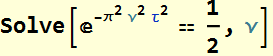
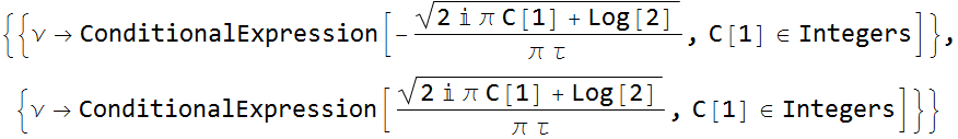
Its half-max width can be obtained by solving: 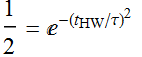      (1.2)

Let C[1]=0, for Re solution, then   (1.3)

Now, let’s take its Fourier transform:

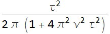
The Fourier component spectrum is:       (1.4)
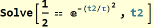
Its half width can also be solved:

Again, let C[1]=0, 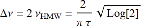  (1.5)

Hence, combining (1.3) and (1.5)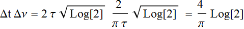  
which is constant, independent of τ
Also:                                         (1.6)

We can plot it out on a log-log plot.

Constant (pulse duration) x (spectral width) is a fundamental property of Fourier transform.

Laplace pulse

Consider a Laplace pulse:                                (1.7)
Its half width can be obtained by solving:           (1.8)
Or:                                                      (1.9)

Now, we obtain the FT:

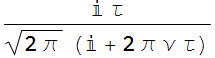
We are interested in its magnitude, hence, take the amplitude square:

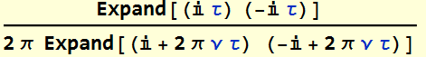
The peak value is at ν=0:

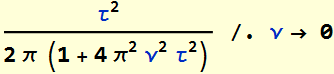
The frequency at half max is:

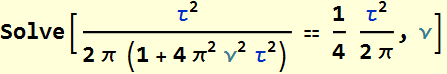
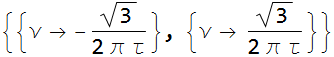
Hence,                                               (1.10)

Combining (1.9) and (1.10)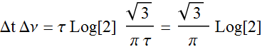  
Again, (Δt Δν) is a constant.

1.2 (15 pts) Transform-limited concept

The pulses you did above are transform-limited (the time domain and the spectral component are Fourier transform of each other), which means that the product Δt Δν of pulse duration Δt and Fourier spectrum bandwidth Δν is the minimum possible.
Can we have a pulse with Δt Δν >> the transform limit? (just word discussion is good enough, but if you can use the App to do demo, you will get extra credit).

Answer

Of course, just have many pulses spreading over a wide wavelength range, or continuous wave with a wide spectrum. Think of sunlight: it spans over the entire visible spectral range and suppose we make a very short pulse out of it, Δt Δν  ~ ∞. It is challenging to make a transform-limited pulse with minimum Δt Δν, there is no limit how large Δt Δν can be.

2. (50 pts) Numerical representation of a pulse

A pulse can be numerically represented with an array:   
of the E-field amplitude over a time range with regular sampling interval Δt

2.1 (25 pts)  Generate an array of number to represent your pulse

Choose your pulse width to be 1.xxxx (ps) where xxxx are the last 4 digits of your student ID.
Choose the time range to be -40 ps to 40 ps.
Select the time interval be 0.1 ps (you will have 800 or 801 data points).
Generate an array signal, name it sE and plot it, using the help below.

Answer

Below is the answer for all pulse types. You are asked to do only for your pulse type.
Run the code below and put in appropriate parameters for your answer. There are more than one way to write the code, you are encouraged to write your own code as long as you obtain correct answers.

Code for numerical array of E field

Here are examples of output from the code above.

2.2 (25 pts) What is the spectrum of your pulse?

Obtain the Fourier transform of your pulse, plot both the Fourier component and its magnitude squared, which is the power density. Explain each result (as if to someone who doesn’t know Fourier transform).

Answer

Run the given code.

Code for a numerical array of E field and its Fourier transform

To get credit, you must interprete each graph of your result. Below are examples.

This is the magnitude Fourier component vs frequency (Fourier magnitude spectrum)
   

This is the squared Fourier component vs frequency (power spectrum or power spectral density)
  

This is the phase of Fourier components vs frequency (phase spectrum)
    

3. (150 pts) Pulse through a dispersive device or system

Finally, we get to the point: If you have a pulse transmitted or reflected from an optical device/medium/system, what will happen to the pulse?
“But what do you mean what will happen?” At first, the question may not even make sense to you, right? what happens is this:

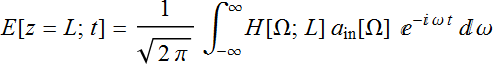
The pulse is not made up of just one single frequency, but is a linear superposition of infinite frequencies, which is expressed mathematically:
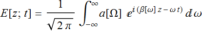                                (Eq. 3.1)

Each frequency has its own frequency response function (be that transmission or reflection or any output from a  device or system), which is frequency-dependent. In other words:
                                         (Eq. 3.2)
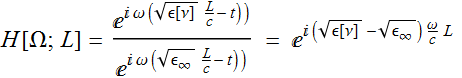
where H[Ω] is the frequency response function of the optical device/medium/system. Realistic device also has β[ω] medium dependence. But for the sake of simplicity, we consider the case of reflection only, where β[ω] of incident and reflected field is the same.

3.1 (20 pts) Output E field expression

Based on Eq. 3.1 above and the discussion followed, write a mathematical expression (a formula) for the output E field.

Answer

The output E field is:
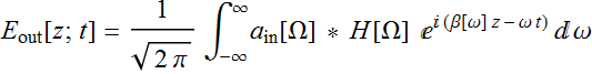                           (Eq. 3.3)

3.2 (20 pts) Reflectivity bandwith of a fiber Bragg grating

Close all Apps not relevant to his HW, and run only the Bragg grating App. (shown below). Click on various icon to read and follow.  If you have a hang-up when open an app, goes to Evaluation, disable Dynamic Updating and after the app starts, make sure you enable it again.

Select the default example: , which is a typical fiber Bragg grating (You can google search to read more on it, but not needed for anything here). The default example here has a very small index difference between the 2 layers of each period: 1.482 vs. 1.480, a difference of only 0.002, and the grating consists of 4000 periods.

     

This structure acts like a mirror, but it works for only a very small range of wavelength around the center wavelength. Based on what you observe, over what range of wavelength that it acts like a ≥ 99% mirror?

Answer

As shown in the graph below, the range for >=99% reflection corresponds to 1-R <= -20 dB, which is ~ 0.9996 to 1.0004. But any answer from 0.999 to 1.001 will be accepted although not accurate.

Code for cursor placement (move the cursor to estimate the range)

3.3 (20 pts) Reflectivity of a pulse from a fiber Bragg grating

For this quesion, you need to run the app below, concurrently with the Bragg grating app above. These 2 apps are designed to work together concurrently. Close all other unnecessary apps, including deleting any unneeded active Manipulate loop. (Occasionally, you see Mathematica errors because of multi-thread processing, don’t worry, you can continue and it will work, or just close everything and start fresh).

What happens if your pulse spectrum bandwidth is wider than that of the mirror? You can use the App to try out a pulse that most resembles (use your judgment) the pulse you design above, then compare the pulse bandwidth vs. the mirror reflection band. Below is an illustration.

This illustration uses a short-duration trapezoid pulse. We see that its bandwidth (purple in middle graph) is wider than the mirror (blue/teal color) in the middle graph.  
   

Discuss what you think will happen to the reflected pulse? Will it look exactly like the original input pulse? or is it altered (distorted), and qualitatively explain why (see the third graph). All the pts of this question is ALL about your discussion and explanation. You must do it earnestly to get the points.

Answer

Below shows the use of the App for Gaussian pulse.

Below are close-ups of the result.

To understand how the pulse shape changes, consider the output pulse Fourier component:
                                           
where is the input Fourier spectrum, which is represented by the magenta color curve in the left graph, H[Ω] is the frequency response function of the Bragg grating, which is represented by blue/cyan in the left graph. The resulting is yellow in the middle graph, which is obviously different from (pink/magenta). Note that in this example, the center of the Bragg reflection spectrum is set slightly off to the left of the pulse spectral center. You can and should move the Bragg detuning left and right to observe what happens to the output pulse shape.

In the 3rd graph, the output pulse shape, which is obtained with the inverse Fourier of and shown as the greeen curve in the right graph must be different from the input (orange) because    .
In other words, it is distorted from the input, and this example shows a very significant distortion. Below is another close-up of the distortion.

The input pulse is transform-limited, which means Δt Δν is at a minimum. Any distortion would result in larger Δt Δν. Since Δν can only be smaller and not larger, it means the pulse can only be broader as shown above.

What happens if H[Ω] is nearly a constant over the significant range of ? If that is the case:
                                           
where h is a constant, then the output pulse shape is the same as the input, and the only difference is factor h.
Below is the same example as above except that the index variation of the Bragg grating is larger to have a wider reflection bandwidth.

3.4 (50 pts) Reflectivity of the pulse you design above.

Now we get the to the heart of the matter: can you do a calculation to find out the shape of your reflected pulse that is designed in Prob. 2 above? At this point, you can close this app (because you will do what this app does).

close this:   

What you need is the frequency response function H[Ω] of the Bragg grating. Run the code below to get the response function in the form of an array named hBM:

Do the rest: calculate the reflected pulse and plot it to compare with input pulse? See hint below

Answer

Numerically, the Fourier transform in problem 2 above is eFFT.
The output Fourier spectrum is the product of input Fourier eFFT and Bragg grating response function hBM

If you execute the code in Problem 2, run the Bragg mirror App above, then the code below should work and that is your answer.

If you get the code above correctly, below is the plot.

Below is a slightly more sophisticated code to allow you varying the scales of the graphs.

code for calculation the pulse envelope output

3.5 (40 pts) Reflectivity from a broad-band mirror

Back to this app (if you closed it, open it again)

Now, select the mirror example: . This is opposite to fiber Bragg grating. The difference between the index can be quite high, and few periods are needed to have ~ 100% reflectivity.

you can choose any value of low index refraction, then choose a Δn value such that your high index - low index=0.4xx where xx is approximately the last 2 digits of your student ID.

For example, in the above, we have nlow=1.45, nhi=1.88652, then Δn=nhi-nlo=

If your student ID last 2 digits are approximately 36, then it is good enough (just close is good enough).
Select the number of periods be 20. What is the range of wavelength that refects >99%? If this range of wavelength is much larger than your pulse, what do you think the output pulse? does it suffer significant distortion like the case above?
Run a code that demonstrate your point.

Answer

The answer for this is essentially given in 3.3 above, except that you should select Bragg mirror option instead of waveguide Bragg grating option. Below is the recap. All you have to do is to illustrate the case of your pulse with the Bragg mirror option.

4. (50 pts bonus) Pulse through an absorptive medium

Do this if you enjoy it for your own learning, or to catch up if you missed a lot of stuffs we did in the class.

Consider an absorptive medium with a single-oscillator Lorentzian profile. Can you calculate what the output pulse looks like?
Note that this is the reverse of the case of Bragg grating in Prob. 3: Bragg grating reflects, or preserves the pulse central spectrum, but cuts off the wings. This case cuts off the central spectrum and leaves the wings less affected.
The problem is illustrated below. Suppose we we have a short pulse (blue) entering a region of a medium containing atoms or molecules (red dots) that act like a single Lorentzian oscillator at the pulse carrier frequency. What is the shape of the output pulse? (neglecting the reflections at the region boundaries).

illustration

Complete answer

Note: The original problem asks you to do only 1/2 of the work by asking to consider only the amplitude part  {H[Ω]} of the response function H[Ω] (The answer you obtain would be only “half-way”). Here, we will do the whole thing by using the complete H[Ω] with both amplitude and phase.

4.a Constructing a dielectric model for a single Lorentzian oscillator

The dielectric constant of a system with N Lorentzian oscillators is given:
                                 
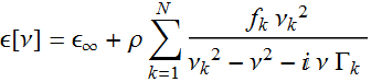
  where:
       -   is the resonance frequency of the   oscillator,
       -   is the linewidth of the   oscillator,
       -   is the oscillator strength of the   oscillator, and
       - ρ is a relative density coefficient, which can be set =1 if the medium is 100% made up of the oscillators and less than 1 if the oscillators are dopants (or admixture) in a neutral medium.

Below is a model for a dielectric with a single-Lorentzian-oscillator, N=1. The app allows choosing via its wavelength ,

4.b Optical pulse through the medium

The E-field wave of frequency ω traveling in such a medium is given:
                    (we define  )         
Denoting:     ,
we can write:
                    
where we define:      .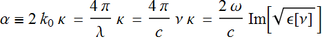

The frequency response function H[Ω] is the ratio of the input at z=0 vs output z=L (the travel length in the medium).
                          
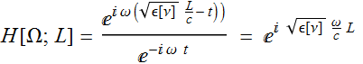
However, note that we are NOT interested in the part of change that is due to the background medium without the oscillator. The more relevant response function is the change with and without the oscillators, which means:
                           

Hence, the output signal is:
                            

We have to apply the above formula in numerical computation.

4.c Numerical implementation.

For the coding, everything is the same as above, except for H[Ω].

Step 1: Code for pulse and its Fourier transform

Step 2: Code for the transfer function, including detuning option, show

Step 3: Inverse Fourier to get pulse out vs. time

4.d Put all together into a single app

We can put all three steps above into a single app below. (Not required - this is only for your learning).

An example of the app is shown below.