HW 8B Study guide
Topic: dispersion in materials

ECE 5368/6358               han q le - copyrighted
Use solely for students registered for UH ECE 6358/5368 during courses - DO NOT distributed (copyrighted materials)

Introduction

As we discussed in class, dielectric optical materials have a wide range of refractive index, and the variation of index vs. λ is what gives us the prism effect and rainbow. The purpose of this HW is to explore a little more into this topic.

Background learning materials

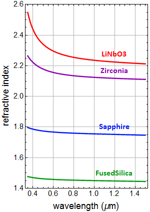
Look at the graph above. It is plotted using the Sellmeier model (or equation) for material dielectric:
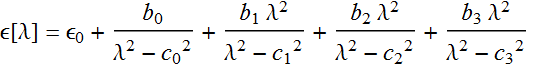                          (1)
The refractive index is obtained as:         (2)
where subsript “ph” indicates that this is the phase velocity index.

The coefficients b’s and c’s in Eq. (1) are obtained empirically, i. e. they are whatever values that fit the experimental measurement of a material. (Alternatively you might find the equation is sometimes expressed as:
      
which is the same).

Later on, we need to find the group velocity, which is defined as:
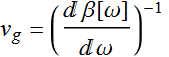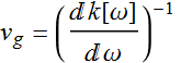                              or                 (3)
Starting from the relation:
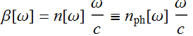                                                     (4)
we see that: 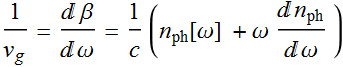                          (5)
Hence, define the group velocity index :
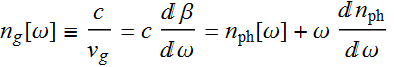                                    (6)
Since the data for is expressed vs. wavelength, it is convenient to use λ as a variable:
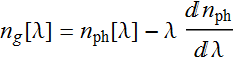                                                         (7)
in which, we use the differential relation:    
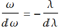                                   because:              (8)

Later on, we will also need the group velocity dispersion or GVD, we use the formula:
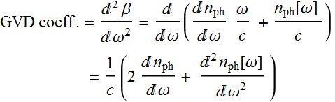                          (9)
It is more convenient to express in terms of wavelength:
                          
                                                (10)   

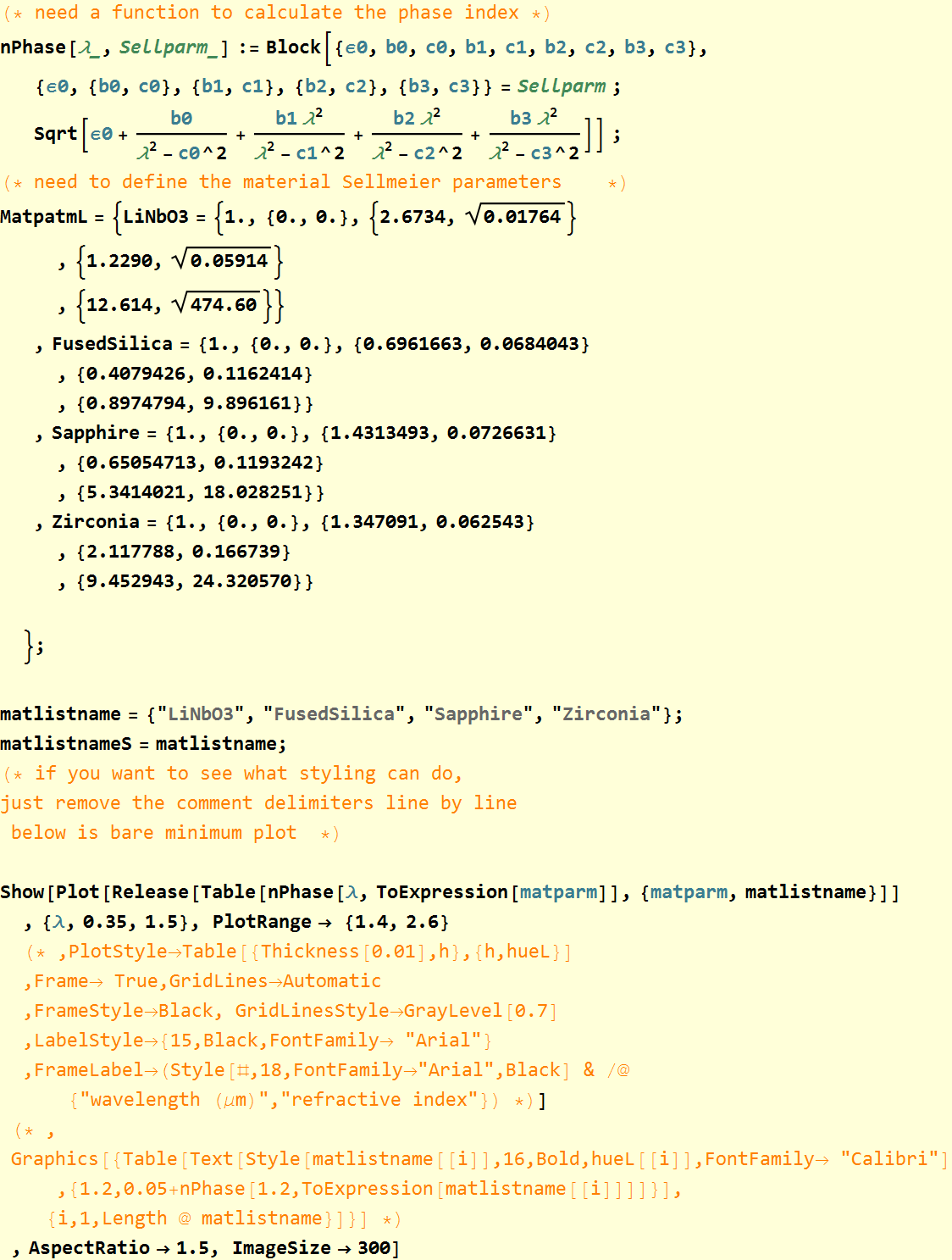
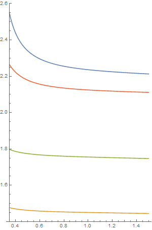
1. (40 pts) Material refractive index

Below are the coefficients of the 4 materials displayed: (lithium niobate), fused silica (high quality glass), sapphire, or zirconia.
(If you wish to know more, go to this web page for information about the refractive index of various materials. There are other sources, and don’t worry about slight discrepancies between various sources. All these are empirical data and slight differences are to be expected).

data presentation

LiNbO3	1.	0.	0.	2.6734	0.132816	1.229	0.243187	12.614	21.7853
FusedSilica	1.	0.	0.	0.696166	0.0684043	0.407943	0.116241	0.897479	9.89616
Sapphire	1.	0.	0.	1.43135	0.0726631	0.650547	0.119324	5.3414	18.0283
Zirconia	1.	0.	0.	1.34709	0.062543	2.11779	0.166739	9.45294	24.3206

1.1 (15 pts) Plot  

You should get a similar chart above. No need for elaborate style.

solution

code

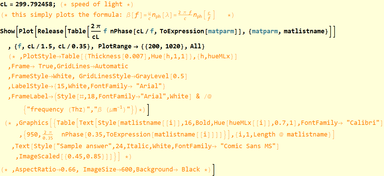
1.2 (15 pts) Plot  β[f]

Calculate and plot the propagation coefficient β[f], which is given as:
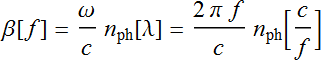                where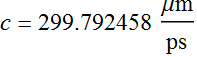    
for λ from 0.35 to 1.5 μm. (This is just a step to encourage you to use the computer and any software you like, including Excel to do calculation and plotting). Below is the answer so that you can check.

solution

code

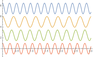
2. (20 pts) Wavelength

Plot the E field of a unity-amplitude planewave in these 4 materials propagating in z-direction at λ=550 nm.
That is, plot           
However, you don’t have to animate, just plot as a function of z over a distance of 3 μm.

Solution

code

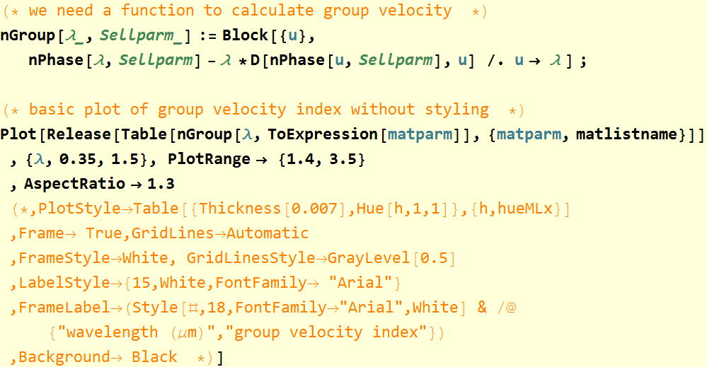
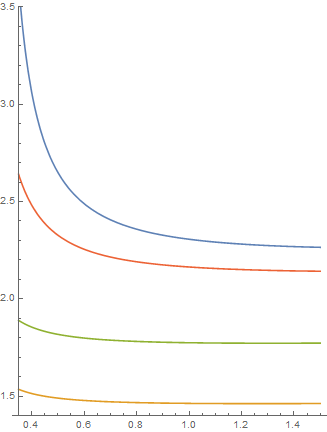
3. (20 pts) Group velocity

Group velocity is defined to be:  . β[ω] is what calculated in Problem 1 above.
Group velocity index is defined to be:   (see more in “Background learning materials” in the Introduction).
Plot group velocity index for these 4 materials as a function of wavelength, and put this plot side-by-side with the phase velocity index plot (which is what we called refractive index) as shown in the chart at the introduction. Are there any differences between phase and group velocity indices?

Solution

Code

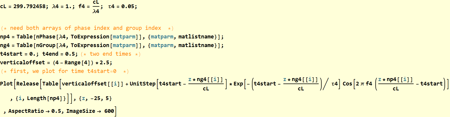
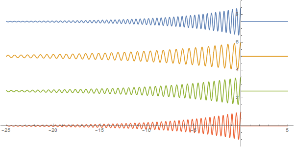
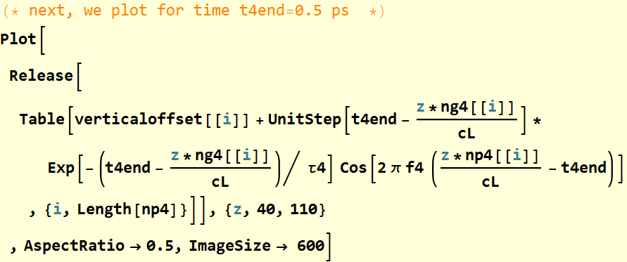
4. (60 pts) Pulse in different materials

Consider this pulse shape envelope: . It looks like this:

We discussed in class that the E field for such a pulse shape with carrrier frequency is given:
                     
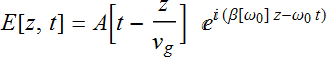
if we neglect the group velocity dispersion. Let τ be 50 fs. Plot the pulses for λ=1 μm in the four materials at:
- t=0: make all 4 pulses lined up with the leading edge at z=0
- t=0.5 ps. (the purpose is to show the pulses travel different distance in different materials).
No need to animate. Just plot the pulse in space along the z-axis. Choose a z-range that contains more than 95% of the pulse energy.

Solution

Code

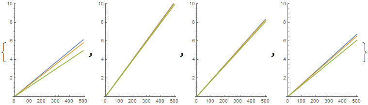
5. (20 pts) Pulses of different wavelengths

Consider three λ’s: 0.65 μm, 0.532 μm, and 0.405 μm. Neglect the GVD effect on the pulse shape, plot the pulse position as a function of time from 0 to 500 ps for each material. Here, the pulse shape is irrelevant as we neglect the GVD shape distortion effect. All pulses move with group velocity. No need for animation.

solution

code

6. (40 pts) Group-velocity dispersion

Plot the group velocity dispersion defined as:    for the 4 materials above as a function of wavelength from 0.35 to 1.5 μm. See the Introduction section.

solution

code