Noise and Signal
ECE 6323            H. Q. Le Copyright
Only for students of ECE 6323/5358/6358 - Do not distribute

1. Noise basic concept and Power Spectral Density function

1.1 Introduction

Example 1

We measure some quantity as a function of time or space, or whatever. Our measurement is a set of numbers like this: (it has 50 elements):
{7,6,12,9,15,13,9,11,9,10,10,6,9,11,11,8,10,11,10,3,17,12,12,10,13,11,15,7,14,
  13,10,10,9,9,18,10,6,12,9,7,10,6,13,7,10,9,6,11,12,12};
We can plot our measurement like this:

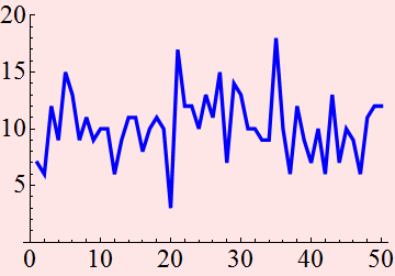
The signal is not constant, but fluctuates a bit. What is the meaning of this fluctuation? is it meaningful? or meaningless? Does it contain information or not? There is NO WAY we can answer this question beyond a shadow of doubt. But if we don't find this variation with any useful information to us, we call it NOISE.

So, we define the concept of noise, but how do we describe it? Suppose we do the measurement again and this time with get the result like this:
{10.19,9.743,9.734,9.811,9.796,10.43,9.606,9.965,10.26,9.973,10.09,10.22,
  10.48,10.4,10.23,10.24,10.26,10.29,9.917,10.17,9.816,9.457,10.26,9.432,
  10.18,9.749,10.06,10.32,9.545,9.924,9.841,9.427,9.716,9.922,9.604,9.956,
  9.68,10.15,9.877,10.1,9.799,10.67,10.65,10.31,9.892,9.923,9.999,10.1,10.,
  9.543}
  Let's compare the previous signal with this:

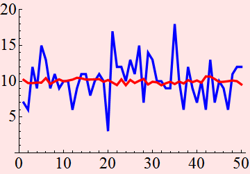
We would intuitively say that the red is less noisy than the blue. But how much is less noisy? how do we quantify the "noisiness"?

1.2 Statistical perspective

Suppose that we KNOW THAT THE QUANTITY WE MEASURE IS SUPPOSED TO BE CONSTANT, then the fluctuation we see is definitely by definition, noise. We can plot the histogram like this

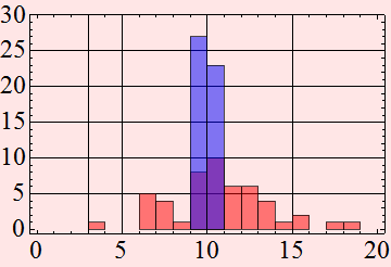
They are so different. We can estimate the mean and variance

Clearly, both signals have very similar mean, but one has a much smaller variance than the other. So, in this case, variance is a measure of the noise.

Can we always use variance as a measure of the noise?

Example 2

Suppose we have a new signal that looks like this:
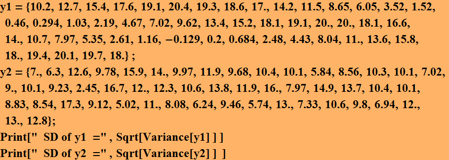
y1={10.2,12.7,15.4,17.6,19.1,20.4,19.3,18.6,17.,14.2,11.5,8.65,6.05,3.52,1.52,
  0.46,0.294,1.03,2.19,4.67,7.02,9.62,13.4,15.2,18.1,19.1,20.,20.,18.1,16.6,
  14.,10.7,7.97,5.35,2.61,1.16,-0.129,0.2,0.684,2.48,4.43,8.04,11.,13.6,15.8,
  18.,19.4,20.1,19.7,18.} ;
  and
  y2={7.,6.3,12.6,9.78,15.9,14.,9.97,11.9,9.68,10.4,10.1,5.84,8.56,10.3,10.1,7.02,
  9.,10.1,9.23,2.45,16.7,12.,12.3,10.6,13.8,11.9,16.,7.97,14.9,13.7,10.4,10.1,
  8.83,8.54,17.3,9.12,5.02,11.,8.08,6.24,9.46,5.74,13.,7.33,10.6,9.8,6.94,12.,
  13.,12.8};
  we can find their variances:

So should we say that y1 is noisier than y2?

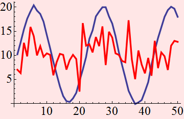
In the above, y1 is blue (variance= 50) and y2 is red variance is 9.8. Their means are:

Again, similar mean. Is it correct to say that y1 is noisier than y2?
This depends! If both y1 and y2 are supposed to be constant, we say that y1 fluctutates more and thus, noisier than y2. On the other hand, it is clearly that the fluctuation of y1 is somewhat predictable, and if we remove this "predictable" fluctuation, it may be less noisy. Thus, this is a key concept: noise BY DEFINITION CAN NOT BE DETERMINISTIC: in other words, noise has to be defined as the unpredictable, indeterministic part of the signal. One way to see in this example is to Fourier transform the signal.

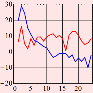
What we plot here is the Fourier transform square, on Log scale (unit dB) of the signal. It is clear here, that the blue (y1) has  a periodic signal at bin ~ 2 that is much stronger than that of the red, and the y1 F-transform signal at higher frequency is actually less than that of y2. In other words, the blue (y1) has a large variance, but seems less noisy than the red (y2).
We see how useful Fourier transform is.
Let's do the follow: we define a new signal y1new that is from y1 but subtracted by a known function that we guess to be a sine function:

Now we compare y1new and y2:

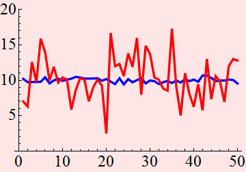
From this, we have to say that y1 is less noise than y2! because eventhough it has a large fluctuation, we deterministically know exactly one component of that large fluctuation, (the sine function) and thus, it can be removed.

Example 3

Now we have a fairly complicated signal that looks like this:

How do we analyze this? well, we can Fourier transform again:

What do we see? is there a signal in there? how much is the noise. Intuitively, we see 2 big peaks that stand out above the rest. We would call those peak signals, and the rest, noise. But what are we doing here, plotting the square of the Fourier transform of the signal? what is the meaning of this? Why are we doing this?

1.3 Power spectral density function

1.3.1 Definition

We define the power-spectral-density function of a signal s(t) as:  
          

This is an important definition. To see what it does, let the signal be:  
; then

Therefore:

Because
In other words, the PSD function of this signal tells us that it is zero for all frequency except for where it is a delta function with an amplitude factor . That's why we call it PSD: it is a measure of the density of the spectral content of the signal as a function of frequency.
The total power is finite:

(the power density is infinite at because the signal has purely frequency)

1.3.2 Practical calculation of PSD

If we have a finite series of signal measurement (or sampled points): , how do we find its PSD?
Let say the series are measured with regular interval (either time, space, or whatever variable we used), then the series actually represent pairs of number:            
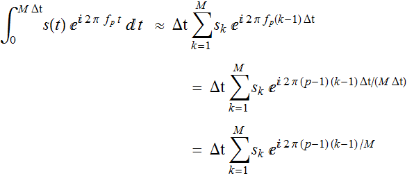
where Δt is the sampling interval. We can take the Fourier transform of this numerical series by approx. the integral as a summation:

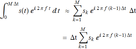
But if we discretize the variable f also, as a series (p-1) Δf for integer p, and choosing  Δf =1/(M Δt), we have the following expression:

But we recall that in fast Fourier transform numerical technique, the Fourier transform of a list of length n is defined to be
Therefore, the above expression can be written as:

This is the basis for numerical calculation. We thus obtain the PSD as:

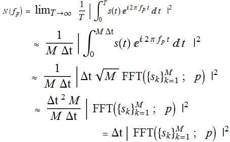
Now we can see why we did what we did: taking the FFT of that data and square its amplitude. Note that the quantity Δt give the unit of 1/(Whatever frequency). If t is time, it is frequency; if t is space, it is spatial frequency, we just call it generally frequency but keep in mind that it doesn't have to be strictly temporal frequency.
So the unit of the PSD is signal^2/frequency. That's why it's call power density.
Some example: if s is E is electric field, ; if s is electric current as function of time, it is .

Example routine

FunctionPSD[x_,DelT_]:=Module[{mx,XFFT,XPSD,fr},

(* first, we take the mean to remove the DC bias *)
                    mx=Mean[x]  ;
(* then we take the FFT of the given series *)                    
                  XFFT=Fourier[x-mx] ;
(* PSD is simply as defined above *)
(* but for real series, we need to take only the *)
(* positive frequency component, which is the  *)
(* first half of the FFT series *)               XPSD=Abs[Take[XFFT,Floor[Length[XFFT]/2] ] ]^2*DelT ;
(* To correspond the PDS with the frequency sries*)
(* we generate the frequency array *)                   fr=(Range[Length[XPSD]]-1.)/(DelT*Length[XFFT]) ;
(* Then, we pair the frequency with its PSD *)
(* and drop the zero frequency component *)
Drop[ Transpose[{fr,XPSD}] ,1]
                    ] ;
LogPSD[x_,DelT_]:= Module[{fr,psd },
        {fr,psd}=Transpose[FunctionPSD[x,DelT]];
        Transpose[{fr,10*Log[10.,psd] }]
                          ] ;
PlotLogPSD[x_,DelT_]:=Module[{lpsd},
       lpsd=LogPSD[x,DelT];
       ListPlot[ lpsd
            ,Joined->True,
    PlotStyle->{RGBColor[0,0,1],Thickness[0.002]}
         , PlotRange->All
           (* , AxesOrigin->{0,-100} *)
        , Frame->True, ImageSize->{450,300}, GridLines->Automatic] ]    

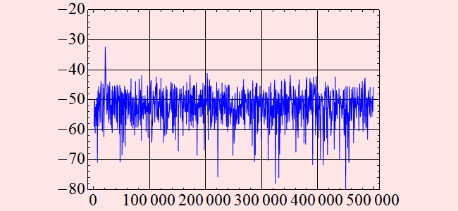
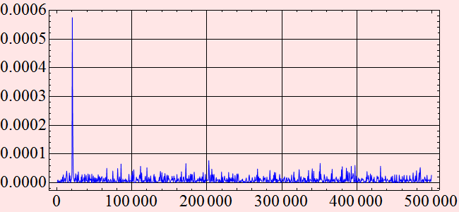
We see that the signal has a component at ~ 20 kHz and at ~ 111 kHz. What is the noise power relative to the signal power? ~ 26 dB and 18 dB, respectively.
The difference between the two strong signals are ~ 8 dB. Does that make sense?
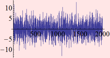
Let's see the way the signal generated:
sig1 = x1+Table[0.5*Sin[x*0.7] + 1.3 *Sin[x*0.13],{x,0,1999,1} ];
        ListPlot[sig1  , PlotJoined->True]
Strong signal amplitude = 1.3, weak signal amplitude =0.5

Indeed it is about 8 dB. What about frequency? we assume the sampling interval is 10^(-6), say sec or microsecond. The frequencies are:

Which is indeed the values we observed. How about our estimation of noise?

The noise looks like the same everywhere: this is what we call white noise, because like white light, it is constant for any color except at the two signals.
We can average them over a range, say, from point 500 to 900:

The noise PSD is about -60 dB/Hz. Where does this number come from?
x1=RandomArray[NormalDistribution[0,1],2000];
This expression tells us that the x1 noise is a normal (Gaussian) distribution with a standard of deviation of 1. The sampling time is 10^(-6) second, or the bandwidth is 0.5*10^6 Hz (remember Nyquist), therefore the power density is:
or -60 dB/Hz.
Let's redo the example above:

compare with

Summary

In general, it can be proven that for a Gaussian process of standard deviation σ, and a sampling interval of Δt, or a bandwidth BW=1/(2 Δt), the PSD is =
or = 2 BW PSD.
The noise is taken as the square root of the PSD:
Noise amplitude = , and its unit is whatever/.

Homework and exercise on noise and signal

Utility package - please execute this

FunctionPSD[x_,DelT_]:=Module[{mx,XFFT,XPSD,fr},

(* first, we take the mean to remove the DC bias *)
                    mx=Mean[x]  ;
(* then we take the FFT of the given series *)                    
                  XFFT=Fourier[x-mx] ;
(* PSD is simply as defined above *)
(* but for real series, we need to take only the *)
(* positive frequency component, which is the  *)
(* first half of the FFT series *)               XPSD=Abs[Take[XFFT,Floor[Length[XFFT]/2] ] ]^2*DelT ;
(* To correspond the PDS with the frequency sries*)
(* we generate the frequency array *)                   fr=(Range[Length[XPSD]]-1.)/(DelT*Length[XFFT]) ;
(* Then, we pair the frequency with its PSD *)
(* and drop the zero frequency component *)
Drop[ Transpose[{fr,XPSD}] ,1]
                    ] ;
LogPSD[x_,DelT_]:= Module[{fr,psd },
        {fr,psd}=Transpose[FunctionPSD[x,DelT]];
        Transpose[{fr,10*Log[10.,psd] }]
                          ] ;
PlotLogPSD[x_,DelT_,Style_]:=Module[{lpsd},
       lpsd=LogPSD[x,DelT];
       ListPlot[ lpsd
            ,Joined->True,
    PlotStyle->Style
         , PlotRange->All
           (* , AxesOrigin->{0,-100} *)
        , Frame->True, ImageSize->{450,300}, GridLines->Automatic] ];
        
PlotLogLogPSD[x_,DelT_,Style_]:=Module[{},
       ListLogLogPlot[ FunctionPSD[x,DelT]
            ,Joined->True,
    PlotStyle->Style
         , PlotRange->All
           (* , AxesOrigin->{0,-100} *)
        , Frame->True, ImageSize->{450,300}, GridLines->Automatic] ]       

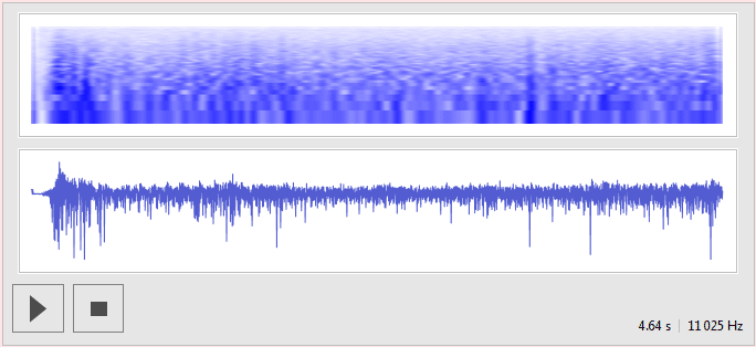
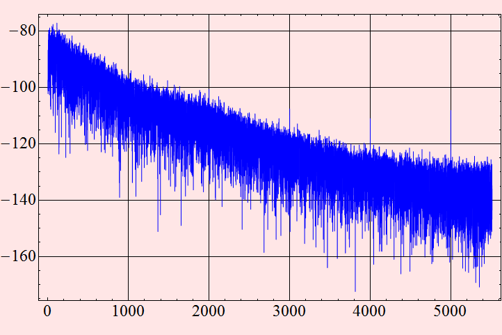
Use your microphone input as signal source

Do the following to simulate signal measurement vs noise using your computer microphone. Play the sound below.

Now, recording some other sounds with noise

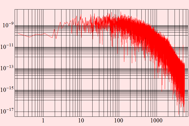
Perform spectral analysis: use the power spectral density function

Now you should compare the different signals - especially their noise level, signal level, and signal to noise ratio.

Signal and noise

Generate some strong noise. Record it and perform spectral analysis.
Generate a signal, something you are familiar with, starting weak. Then increasing noise the signal until you see it above the noise. Determine the NES: noise equivalent signal.

2. Shot noise and related

2.1 Introduction

Suppose we measure the current from a detector or sensor or whatever, and it has a constant dark current (or DC current) even in the absence of the stimulus, . We sample at regular interval Δt. The average number of electrons is:
                                    
where e is the charge. The number of electrons per unit interval obeys Poisson distribution:
                                   
For large , this distribution approx to Gaussian:
                                    
where σ = .
What is the power spectral density of the dark current?

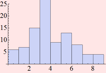
Exercise and Example Poisson

Select a number between 1 and 10. Use it as naverage and enter.

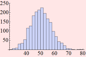
Select a number between 40 and 80. Use it as "naverage" and enter.

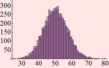
Exercise and Compare Poisson to Gaussian for large mean

Compare Poisson and Gaussian distribution for large mean value: they become similar to each other. Pick a mean value >50.

Do you notice that they become very similar to each other? You can plot them on top of each other as follow:

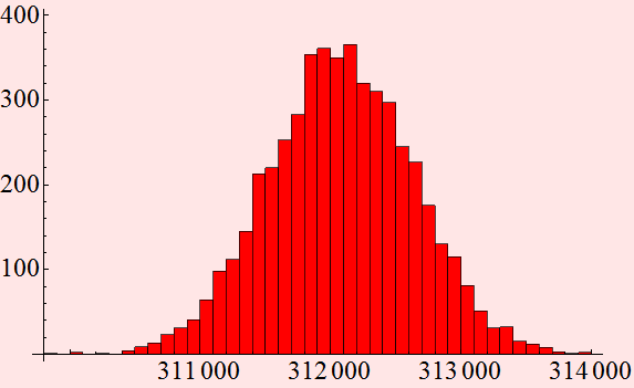
Exercise and Dark current example 1

Consider a PD with 1 mA dark current. Suppose we measure with 20 GS/s, which means that we perform 20,000,000,000 measurements per second, what is the distribution of the electrons in each measurement like?
The mean is:                   
                                        
                                        

What is the noise fluctuation?
                                

The noise current is:

Hence, the current fluctuation is in the order of 1.79 microAmp.
Is this large or small? well, it's all relative.
Consider that we have 0.1 uW signal falling on a detector with 0.5A/W responsivity. The signal would be:
                                            
This is smaller than the noise.

Dark current exercise 2

What is the minimum optical power you can detect with 20 GS/s? (in 50 ps) with the above detector?
Repeat the same calculation as above with sampling rate at 1 MS/s. (sampling time 1 μs)
What can you conclude about noise vs. bandwidth.

Noise current exercise 3

Simulate the current (including noise of course) for a detector with 5 μA dark current for the following cases:
1- sampling at 10 GS/s (10 gigasamples per second)
2- sampling at 100 MS/s (100 megasamples per second)
In each case, calculate the number of average electrons you detect, their fluctuation (standard of deviation). Which case has larger electron (hence current) fluctuation? If so, which case (1 or 2) is noisier? (BE VERY THOUGTHFUL and CAREFUL about this question).

2.2 Shot noise

Even without dark current, any signal also has statistical fluctuation that obeys Poisson statistics:
                                                
                                               
The corresponding distribution of the current measurement is:
                                   
where . Notice that:
                                       
Or:                                            
(remember that 1/Δt = 2B Nyquist); then PSD of this distribution (number of electrons in Δt interval) is:
                                          
Very often, for photodetector, the dark current shot noise is the limiting factor, then people define a noise equivalent power, which is the power that generates a signal = noise.
                                            NEP =
The unit of NEP is __W__
Often, we also scale the NEP per unit of , hence the NEP/ is:
                                            NEP =
The unit of NEP per bandwidth is __W/_____
and the detector detectivity is define as:
                                            
For semiconductor PD, the dark current is proportional to the detector area, thus, people define a specific detectivity by scaling D vs. detector area :
                                          
The unit of specific detectivity is thus:  .
Notice, in some case, you may see this (without the factor of 2). It is just a matter of convention about the noise power (just one band or both bands).
                                    

Use the formulas given above to calculate the detectivity for a detector with a dark current of 0.5 nA, and responsivity of 0.65 A/W

If you are trying to detect a 10-nW signal, and suddenly, someone turns the light on in the room with 10 mW of ambient light falling on the detector, what is your SNR?

2.3 Optical quantum noise

Similar to electronic shot noise, we can have statistical fluctuation with photons. However, photon statistics is more complex when they are in certain quantum states. Neglecting these cases of quantum coherence, we can treat most other cases with Poisson statistics.
Suppose we have a stream of photons with an expected average within some time interval Δt. Then probability of detecting n photons is:
                                                    
But this is what we detect, it is NOT necessarily the statistics of light from a source, since we don't know the source characteristics, i. e. how it emits light.
For quantum-incoherent light emitters, the intensity distribution is actually:
                                                    
Thus, the photon statistics from such a source is obtained by averaging over the Poisson distribution, which yields:
                                                       
This is known as Bose-Einstein distribution.

Example, let nave=9, this is the distribution:

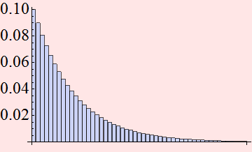
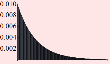
Here is with larger nave.

2.4 Theoretical digital signaling quantum limit

Discussion

If we have a perfect detector, one that gives us zero dark current, and 100% quantum efficiency, and we use it for optical communication, do we have the probability of errors?
The answer is yes! this has NOTHING to do with how perfect the detector is, but the fundamental quantum process of detection. Remember from above, suppose we have a pulse of light with an expected average , we don't actually detect , but can be any number n with the probability:
                                                      

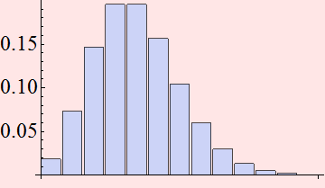
We see that there is a finite probability of error: we may detect no photon while in fact there is an average :
                                              
Suppose our system is digital, so that if there is one photo-electron, we call bit 1 and without it, we call bit 0, then in fact we have an error when we detect 0 photoelectrons. In other words, we miss a bit 1 signal.
Hence the probability of error is:
                                                 

Bit error rate

We define bit-error-rate (BER) is the fraction of error of all the bits. Hence, a BER of means that out of one billion bits, we may expect 1 bit error. Notice that we say "expect" only, not guarantee that there must be one bit error. We may have more or less, but the ensemble average is 1 bit of error in one billion bits.
Now, given the error above, what is the BER as a function of ?

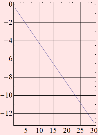
So, for a BER of , we need at least:
                               

Or 20.7 detected photons. Of course, this is the quantum limit for ideal receiver. Realistic system is a lot worse than that as we will see.

Example: For 10 Gb/s and a wavelength 1.55 um, how much power we need for an error rate of 10^-9?

The number of photons per bit:
                                  
The number of photons per second:
                                   
The power is:              

A mere 27 nWatt. In dBm, it is:

A useful physical constant is:

Or -46 dBm.
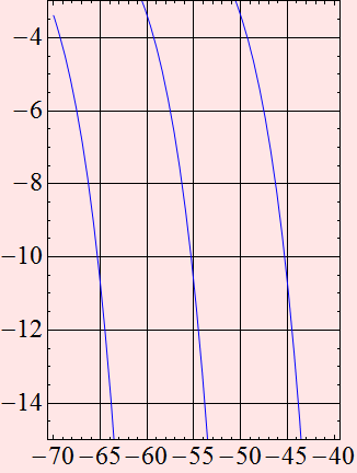
A chart we often plot is the BER as a function of power for a given BR:
                                     
      

As we can see, we obtain the value of BER as expected.

2.5 Theoretical analog signaling quantum limit

Comparison of important parameters between DIGITAL and ANALOG
                             DIGITAL                              ANALOG
                              BER                                     Signal-to-noise ratio (SNR, S/N)
                              photons/bit                           Photocurrent
                              Discrete signal (1,0)             Continuous
                              Bit rate                                 Bandwidth (analog)                                  
The signal of analog system is not bit, but signal current (continuous), . The noise is                             
                                                         
The signal to noise ratio (SNR) in terms of current is:
                                                    
There is another definition of SNR that is in terms of signal power, not current.
Remember that Power < :
                                                  
In terms of incident optical power:
                                                   
Obviously, we are assuming an ideal detector without dark current. Assuming also that the QE is perfect 1,
                                                  

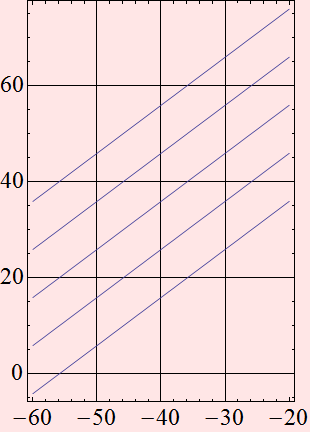
Example plot of signal to noise ratio

3. Other noise

3.1 Johnson (thermal) noise

Electrons in a medium at a finite temperature do not rest, but agitate. Thus, there is a fluctuating current, of which the average is zero, but not the mean square. The kinetic energy of electrons ~ . The noise power is:            
If the curcuit resistor is R, then                  
Or:                                                                                                   

The noise current is ~ 18 nA.

3.2 Relative intensity noise and laser noise

3.2.1 Introduction

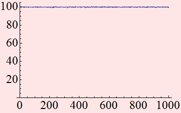
Beyond the light source quantum noise, lasers have other noise sources that come from a number of complex physical mechanisms. One way to describe the laser noise is the concept of relative intensity noise or RIN. As you measure the laser power, for example 1 mW, you will see that it is NOT always exactly 1 mW but fluctuate a little bit. See below.

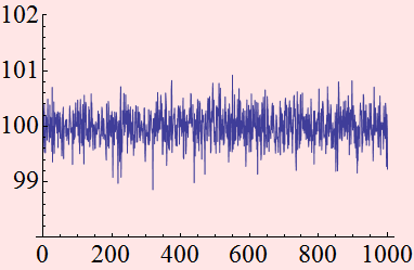
If we take the fluctuation, divide it by the average, we will see the change in percentage. The above curve shows a fluctuation ~ 1%.

3.2.2 General discussion

General concept: Suppose we have a signal S[t] that is supposed to be constant . We measure the fluctuation in terms of its mean value : . We call this relative amplitude noise. If another quantity is a power function of S[t], e. g. , . Thus the power spectral density of relative noise of P[t] is of that of S[t].

Back to laser RIN: a laser source intensity (or power) is not constant, but fluctuates. Sure, we see that at the very least, we have quantum noise fluctuation. But usually, the fluctuation is even much larger than quantum noise. They are called intensity noise. Since it is measured relative to the DC intensity level, it is called RIN: Relative intensity noise
We express the power as: P(t), and let P(t)>. The relative intensity signal is: r(t) = (we can drop 1, which is just a constant with zero noise). Its noise PSD is:
      
Since r(t) is unitless, the PSD unit is usually expressed as dB/Hz. Sometimes, we just use the square root value and still call the same name RIN. How to tell one from the next? look at the unit, whether dB/Hz (power) or dB/ (amplitude).

Understanding RIN is very important to use the laser properly.

3.2.3 Typical laser RIN

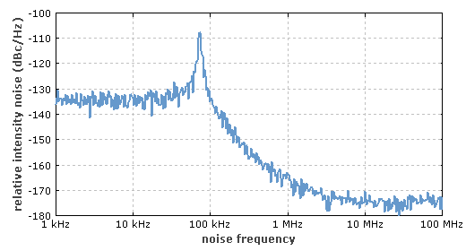
Here is ONLY an example. By no means the same for all lasers. Each laser has its own RIN PSD.

Example: Suppose you purchase a laser diode with a flat RIN of -125 dB/Hz from 10-100 MHz. You want to modulate the laser at 50 MHz. What is the intensity noise do you expect?
                                               
                                               
                                               
                                              

Thus, the relative noise is 0.3976% or ~ 0.4%. This is how much the laser fluctuates at 50 MHz.
If you modulate the laser at 12.5 MHZ instead, what is the fluctuation?

4. Receiver (6323 only - part 2)

Introduction

Link to ppt file - receiver

Response

With voltage amplifier the response is simply the net load resistance, which is parallel between the bias load and the amplifier load
                                   

With transimpedance amplifier:
                                  
where G is the open-loop gain of the op-amp.
The approx 3-dB bandwidth is:
                                        
                                        or:
Notice that gain (given by ) is trade-off with bandwidth. This gain-bandwidth trade-off is very fundamental. Recall the gain-BW product of transistor. Later on we will also see gain-BW product limit of APD.

For other circuits, e. g. p-i-n FET (HEMT) or p-i-n HBT or APD-FET, HBT etc... all can also be modelled generically    where P and Q are polynomials. Often, parameters are obtained empirically.

Noise figure (general discussion)

A very important concept associated with any systems is noise figure. It is most often associated with amplifiers. Suppose we have a weak signal and we want to amplify.
Suppose we have this signal:

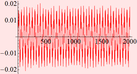
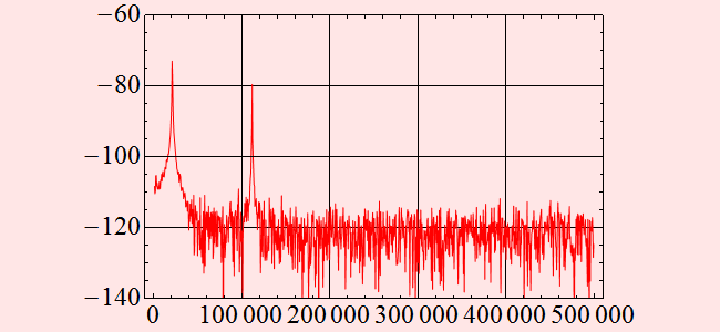
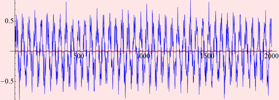
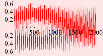
Our amplifier has a power gain of 30 dB. After amplification, we have a stronger signal:

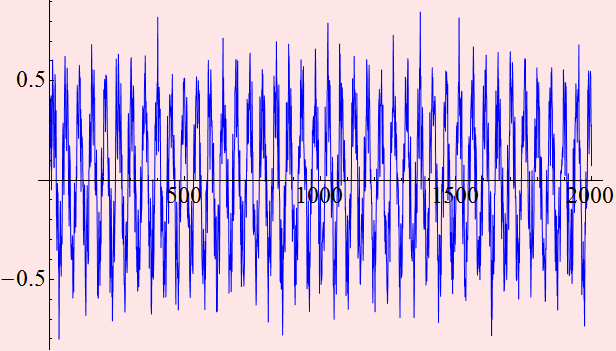
We see that our signal is stronger. It is ~ 0.45 V compared with 0.015 V before, a gain of ~ 15 dB (power gain is 30 dB). Let's compare the signals. Do you think the noise is less for the amplified signal?

We can blow up the first signal to compare with the amplified signal

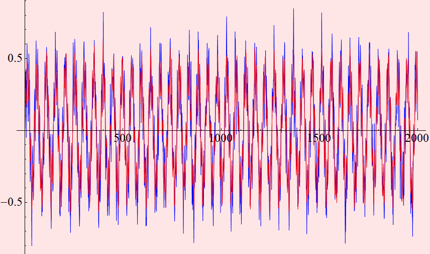
Why aren't the signals exactly on top of each other?
Let's look at the amplifed signal power

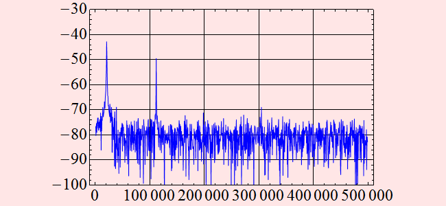
It looks quite similar to the one before amplified, with the only exception that the signal power is higher, ~ -43 dB instead of -73 dB.
Let's compare them on the same scale

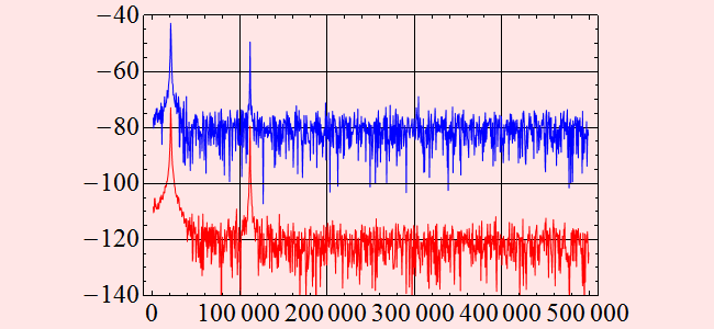
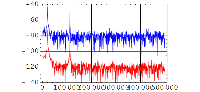
Are they similar with each other except for a vertical shift?

We notice that the signal gain 30 dB in power, but the noise floor seems to gain 40 dB in power. Thus, the signal-to-noise ratios before, 47 and 40 dB, become only ~ 37 and 30 dB. What happens? the SNR is worse! This happens because no amplifier is perfect. All amplifers add some extra noise to the output signal. The degradation of SNR is called noise figure (NF). Noise figure thus has a very specific definition, it's the noise level added to a signal by the amplifer. It is a figure of merit of the amplifier; needless to say, the lower it is the better.

If amplifers add noise, why bother using them?

Noise model p-i-n

Additive noise model

We will follow the additive noise model, which states that the total noise is the sum of the square of uncorrelated noise, which is based on the Gaussian:
                                             
For a PIN receiver, there are 3 effective noise terms: shot noise, thermal noise, and amplifier noise.
Shot noise:                                 
Thermal:                                     
For the amplifier, a most general model is that it is a source of noise that has a series voltage noise and a shunt current noise . Let Y be the shunt admittance of the amplifier, The total noise is an integration of these two over all frequencies within the bandwidth:
                                                    
which is usually done with an empirical model.
The total noise is:
                                  
Very often the amplifer noise   is referred to the input load resistance   for an effective noise power of the amplifier. Then we write:
                             
Then, the term     is treated as a parameter that is characteristic of the amplifier which we call noise figure:
                                   
This is indeed a very common and key concept as discussed above.

SNR

We now can obtain the SNR:
                             

Noise model APD

Excess noise

A most important concept with APD noise is excess noise. When gain is applied, the ideal condition is that:
                                           
where M is the gain. In reality, the noise is higher than the shot noise expected for  , which is:
                                    
We will see that in reality, no amplification or gain process is perfect: there will always be extra noise introduced (see noise figure concept later) on top of the input noise. For APD, there is intrisic random gain process (electron ionization process is a stochastic process with certain probability distribution). This process is intrinsic to the semiconductor and cannot be controlled.
Thus, a theoretical model can show that the actual noise is:
                                        
where x is a parameter that is intrinsic to the carrier and the semiconductor (a complex dependence on electron mass, hole mass, ionization probability... ). Typical value of x is ~ 0.2 - 1 for various semiconductors and carriers.
The SNR of APD is thus:
                                           
where is the noise figure.

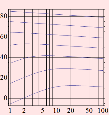
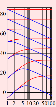
We notice that depending on the signal, there is an optimal SNR for gain. In other words, when the signal is small, we need gain, but not as large as possible. Only certain value of M will give us the best SNR. In fact, we see that:

What if ? Is it possible? Yes.

Indeed, the reason is because of the excess noise factor. Let x=0

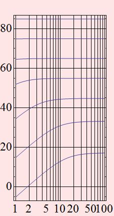
This shows that any gain is good and the larger the better!! Because with gain, we defeat the thermal noise and hence, the larger the better. But because of the excess noise factor, too high gain is counterproductive because the excess noise also grow and cause worse SNR. Infact, compare small x and large x:

More accurate model of excess avalanche noise factor

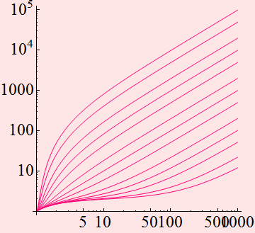
The excess noise factor is actually more complex than just just . It is different for electrons and holes, because they have different transport behavior and ionization rate.
A more accurate model for excess noise factor has the factor different for electrons and holes. For electron:
                                   ;
for hole:
                                  
where k is the ratio of ionization coefficients for electron and hole.
Obviously, k is a very important factor and one can plot

Noise and BER with Gaussian model

If we have a string of 0 and 1 bit, noise can cause error when bit 1 is identified as 0 and vice versa. A threshold is usually set such that if signal S>, it's identified as 1 and 0 otherwise.
For a Gaussian noise model:

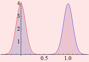
We see that it seems easy to distinguish bit 1 from bit 0 here.

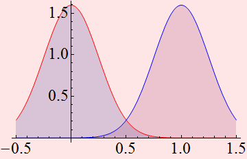
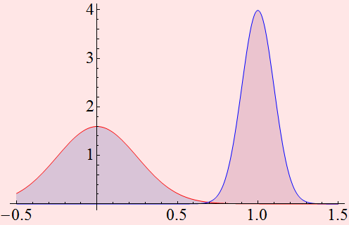
We see now that we really have a problem if the signal occurs near center. We can choose the threshold at 0.5. Everything above is 1 and 0 otherwise. But there is ambiguity. We see that there is a significant probability that we can be wrong. That's the tail end of both distribution.

We can calculate the error rate. This is the error for mistaking 0 as 1 (because the noise make it > 0.5)

Or:
This is the error for mistaking 1 as 0 (because the noise make it < 0.5)

Or:   
Not surprisingly, they are the same because of the symmetry across the line 0.5.
Total error rate is:
                                                   

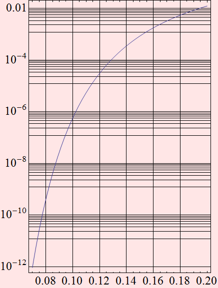
We can express in terms of signal to noise ratio:

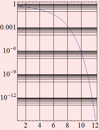
Often, we plot the BER in the reverse log scale:

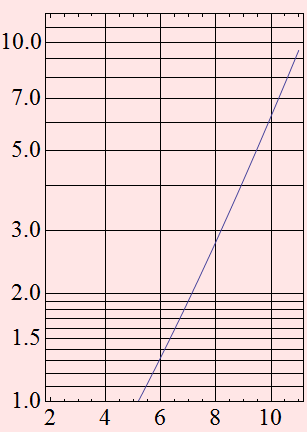
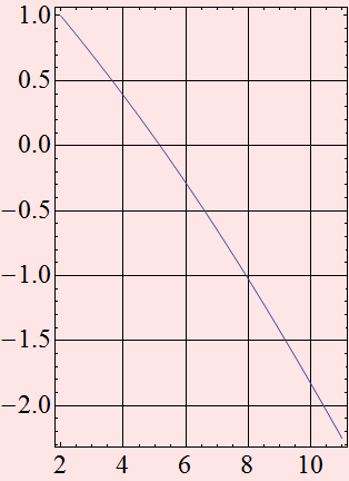
In a bit more details, the noise for 0 bit and that of 1 bit can be different, show how one should minimize error in that case.

Created with Wolfram Mathematica 9.0