ECE 6323 Spring 2014   Mid-term
U of Houston
Han Le - Copyrighted

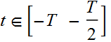
1. (25 pts) Loss in fiber

1.1 Comparing wavelength channels

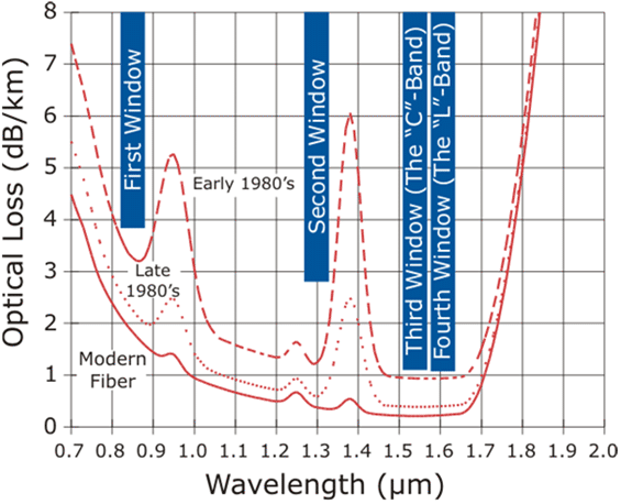
The following signals: 1.55 μm, 1.3 μm, 1.1 μm, and 0.87 μm are launched into a modern fiber (see above) with initial power 1 mW each. Plot their powers of as a function of length from 0 to 100 km on the dBm scale. (all on the same plot) (Use approximate values you can get from the chart by magnifying the figure)  (note: dBm scale is as follow:         )

1.2 Comparing channels - part 2

Do the same as 1.1, but in terms of number of photons on log 10 scale.

1.3 Let the signals now be Gaussian pulses

Let the pulse have a power envelope , where σ=10 ps. As the pulse travels, it also suffers back scattering which means that some of the light is scattered backward, opposite to the direction of its travel. The scattering was both from intrinsic mechanism and extrinsic causes such as fiber structure imperfection.
Let 2 Gaussian pulses of 1.55 μm and 1.3 μm be launched into a 10-km fiber, joined with another segment of 15-km fiber, with a 3-dB reflection at the fiber joint.
Plot the relative intensity of backscattered light as a function of time (over the roundtrip time-of-flight in the fibre). Make also a plot just around the time when the pulses are passing the fiber joint.
Assume that the group velocity effective index is 1.46 for 1.55 μm and 1.47 for 1.3 μm. Assume that there is no reflection at the end facet of the whole fiber.
Hint: see discussion of OTDR below.

1.4 OTDR application 1

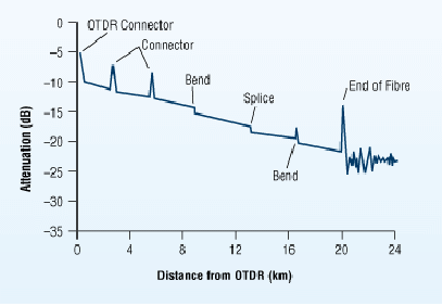
What is done in 1.3 is called OTDR (refer to lectures). By simply converting time-to-distance, we can obtain a plot as shown above. Generate an OTDR plot for your results in 1.3 (simply convert time to distance), and then analyze the result of the plot above to determine the fiber loss coefficient. Notice that a bend and a splice have no “spiky” reflection but just a step drop, discuss the significance of this observation.

1.5 OTDR application 2

Do you think you can indirect;y measure the fiber group velocity dispersion over a wide range of wavelength (e. g. from 1.3 to 1.7 μm) with OTDR? How would you do it?

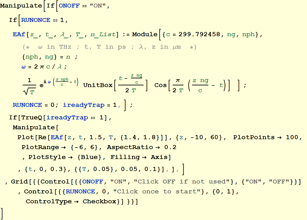
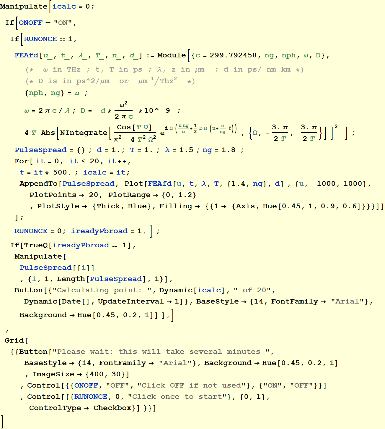
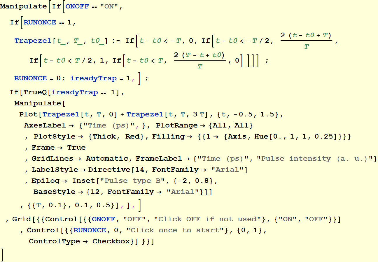
2. (25 pts) Light pulse shape

In the following, use any software you like to do calculation. If you are not familiar with any calculation software, just write out the analytic part and explain how it should be done, then sketch drawing what you think it should look like.

Consider 2 light pulses with a power envelop as given below:
Pulse type A.                                 {t}≤ T
                                                    =0                elsewhere
Pulse type B.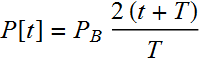                                  
                                                                    
                                                             
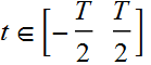
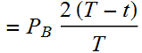
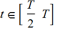
                                                       =0                   elsewhere

This is what they look like:

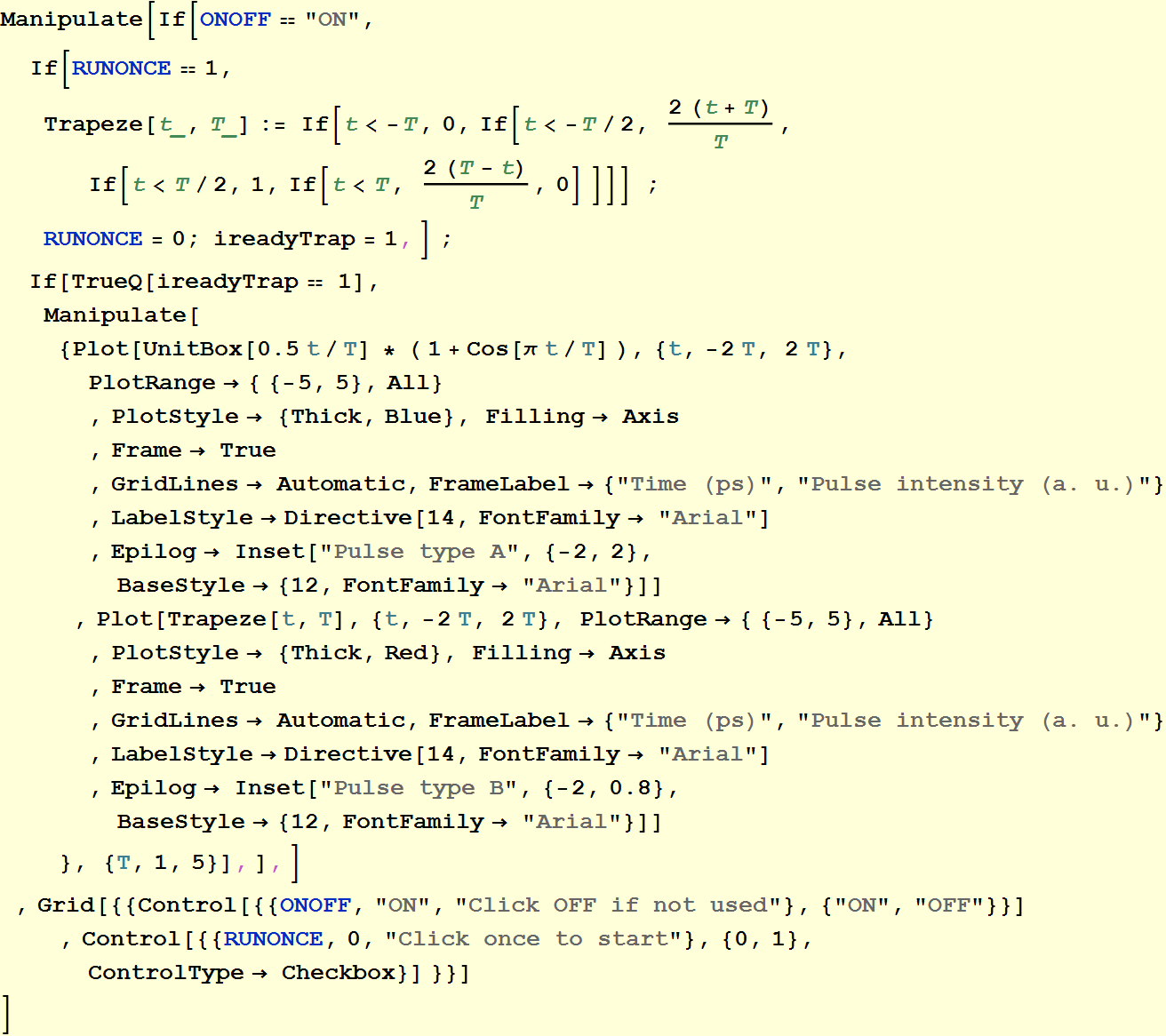
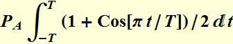
2.1 Normalization

Calculate , and so that the total energy of each pulse is equal to 1: this is called normalization. Plot all on the same plot after you normalize them to compare.

Example

We normalize pulse A:        {t}≤ T

To make , we choose
Hence: 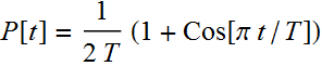                                 {t}≤ T
We can also write:              {t}≤ T

2.2 Pulse with carrier

Suppose you want to use this pulse as an envelope on a carrier . Write the electric field expression for each one of them in vacuum or air (refractive index=1). Remember that they must satisfy the wave equation.
To verify your results, plot the electric field of the traveling pulse (the same way we plot in our lecture); (plot each pulse in a separate graph). We will let the carrier wavelength be 1.5 μm, and let T=0.1 ps. Plotted them over a distance of your choice.

Example

For any pulse, it can be shown that if the E field envelope at one point in space is F[t], then the traveling pulse is:
                                         
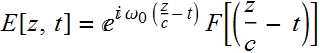
in air or vacuum.  
Example for  pulse type A:
                                      

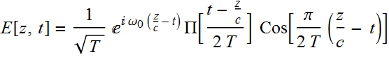
Here is how we plot it:

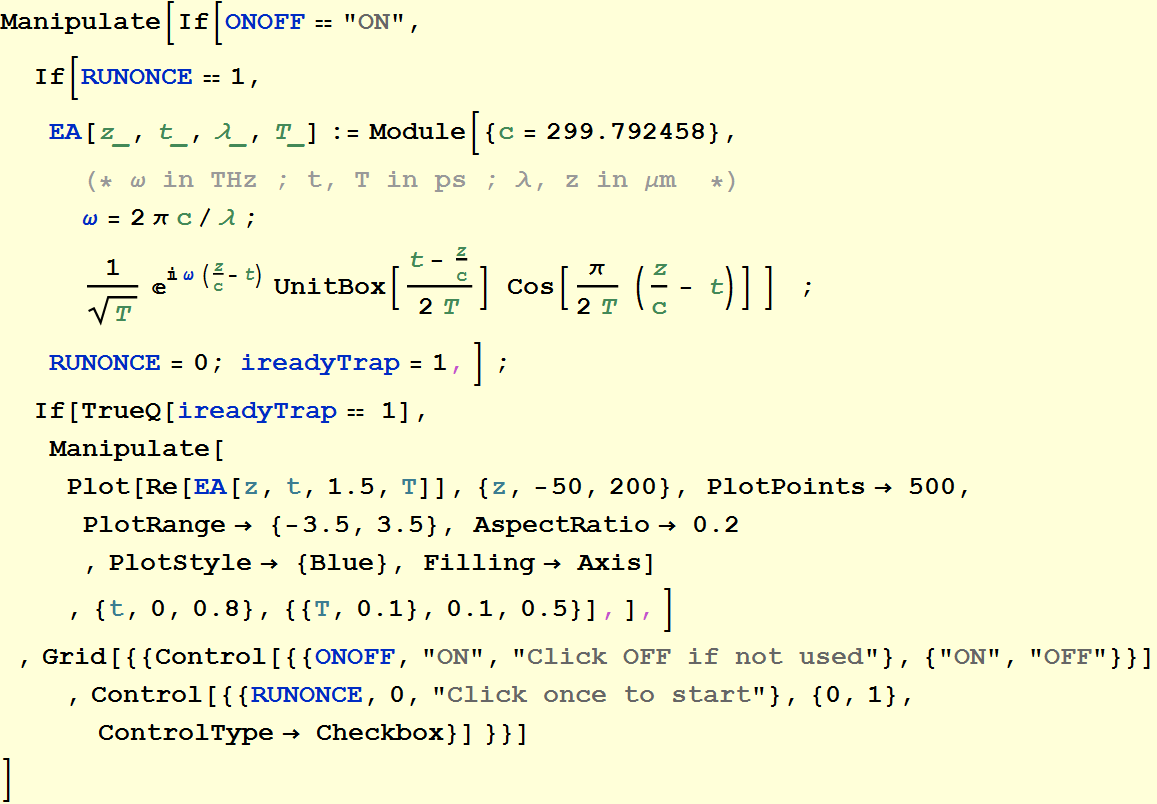
Do similarly for pulse type B.

2.3 Spectrum of a pulse

Calculate and plot to compare the optical spectra of the pulses (plot them on the same plot), using parameters given in 2.2.

Example for pulse type A

The optical spectrum of the pulse is: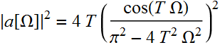    
Here is how to plot it:

Below is a plot in frequency, unit THz

Do the same for pulse type B.

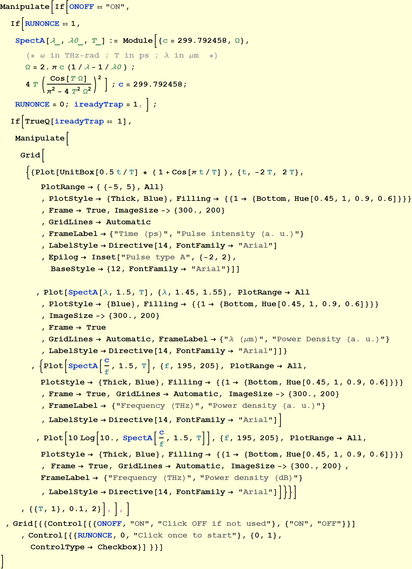
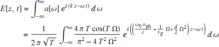
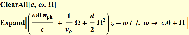
3. (80 pts) Pulse propagation in fiber

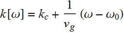
3.1 Group velocity

We have treated the case of no quadratic term and only have to deal with the group velocity for Gaussian pulse. This behavior is of general validity and not just for Gaussian pulse. Do this for pulse type B on problem 2: assume that:
                                               (1)
where:                          ;  
and we refer to as the phase velocity index, which is the same as the modal index. Just for your information, we also define:                 as group-velocity index.
Write an expression for pulse B in problem 2, propagating in fiber given Eq. (1) above.

Example for pulse A:

From the above result:
           

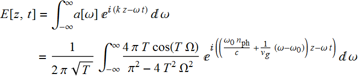
We rewrite:

Hence: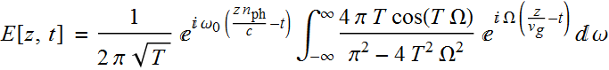         
Use the same result as above:
                     

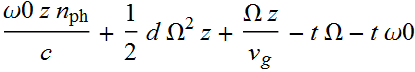
Note that we have a carrier wave that travels with the phase velocity and an envelop that travels with group velocity. This can be prove also for pulse type B.

Derive or write an expression of your best guest for pulse B, then plot.

3.2 Plot to verify

Plot what you have in 3.1 to verify that you get it correctly, use these parameters: λ=1.5 μm, =1.8, =1.4, and T=0.05 ps (we make it very short so that you can see both carrier and envelope. Also we exaggerate . The approx number of cycles in the pulse is 2*0.05 ps x 200 THz= 20 cycles.).

Example

Do the same for pulse type B.

3.3 GVD Dispersion. Plot pulse envelopes as a function of time, assuming you travel with them at their group velocity (see lecture note).

Now, we will include the dispersion term: 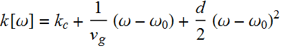                 (2).
You will compare the shape of 2 pulses in Prob. 2: both with λ=1.5 μm, T=0.1 ps as they travel in a fiber. Let d be a variable so that you can put in different values in your plot. Use numerical integration. You should see the pulse broadens as a function of distance, and the larger GVD coefficient d is, the faster is the broadening.

Do this part only if you have  appropriate software and knowledge of numerical method. Otherwise, use your best guess.

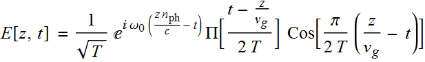
Example for pulse A

The E field is:
               

we have substituted                           

Again, we write: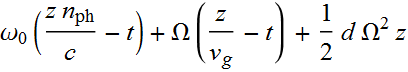    
Then: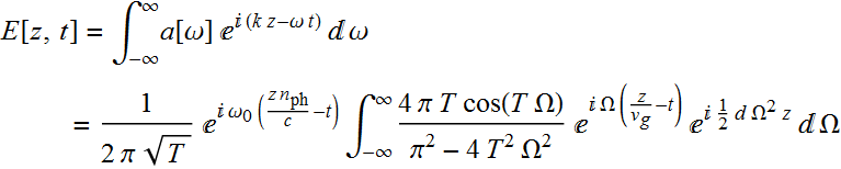              
Since we travel with the pulse, we let :
Then:              
The power envelop is:
                   

Do the same thing for pulse B.

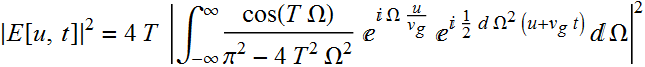
3.4 Plot 2 pulse envelopes of pulse type B that are separated by 0.3 ps as a function of time, assuming you travel with them at their group velocity (see lecture note). You should see them overlapped at certain distance. Use d=1 ps/(nm km)

Do this part only if you have  appropriate software and knowledge of numerical method.

You should see the pulse broadens as a function of distance, and the larger GVD coefficient d is, the faster is the broadening. As a hint, below is the plot of envelop of 2 type-B pulses separated by 0.3 ps (and you can vary them).

4. (20 pts) Laser  - problem 1

See the demonstration below to review concept of laser cavity and modes. Vary cavity length.

4.1 Laser mode 1

A 1.55 μm semiconductor Fabry-Perot laser with an effective index , with 250 μm long cavity. What are the laser longitudinal frequencies (in THz) between 1.53 μm and and 1.56 μm.

4.2 Laser mode 2

In reality, the effective index is NOT constant vs frequency as we have learned. In fact,
         
This becomes:
        
                   
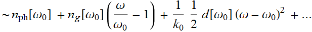
where is the phase and is group velocity index, and d is the dispersion coefficient. Let and   at =1.5500 μm be 3.6 and 3.85, respectively, and . Calculate again the laser longitudinal frequencies (in THz) between 1.53 μm and and 1.56 μm. Compare with results in 4.1 by subtracting to the frequencies and show the differences.

4.3 Laser mode 3

VCSEL has very short cavity. Let a VCSEL have an effective cavity length of 4 μm, and . The gain spectral band is from 1.52 μm to 1.58 μm (very broad). What are the possible laser frequencies? Compare with results in 1.1 and discuss about how to obtain single longitudinal mode operation.

4.4 Laser gain

From the lecture, we know that a simple expression for the condition of laser oscillation is:
                                                
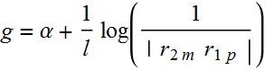
(Look up the meaning of various terms). Let the laser in 4.1 above have , initially. Then one facet is AR coated so that vary from 0.565 (initially before coating) to . Plot the gain as a function of .

4.5 Laser threshold

Assuming that the laser in 4.4 above has a gain-current relation (highly simplified):
                                                 
for current  i > , and . Let  . Plot the change of threshold current as a function of as in 1.4.

4.6 Laser power output

Let the laser in 4.4 has a power slope quantum efficiency 50%. Let its thereshold be 25 mA. Plot the laser power output as a function of current from 0 mA to 100 mA.

5. (50 pts) Laser  - problem 2

Read, search for the original technical document of this article:
http://www.photonicsonline.com/doc/new-laser-brings-faster-internet-0001

(see caltech.edu and google search it).
Describe to the best of your understanding how this laser technology enables higher rate of data transmission. The purpose is only for you trying to critically read and apply various laser concepts we have learned as much as possible. There is no need trying to understand every thing. Just key concept.

Created with Wolfram Mathematica 9.0