ECE 3340 - Extra learning material

The Wuhan 2019 Novel Coronavirus epidemic

Summary

There is a simple approach to estimate the number of Wuhan residents who have exhibited symptoms of 2019-novCoV by using the population of Wuhan residents or visitors who traveled from Wuhan to other countries as a sampled population.

Unfortunately, while the number of infected cases of Wuhan residents/return visitors flying out of China is reported, which is ~140 as of 2/2/2020, the total number of Wuhan residents/return visitors in all these flights are not reported. However, one can make a reasonable assumption about these flier population, such as from 15,000 to 100,000, and calculation can be made to project a range of estimates for the actual number of infected, symptomatic cases of Wuhan residents.

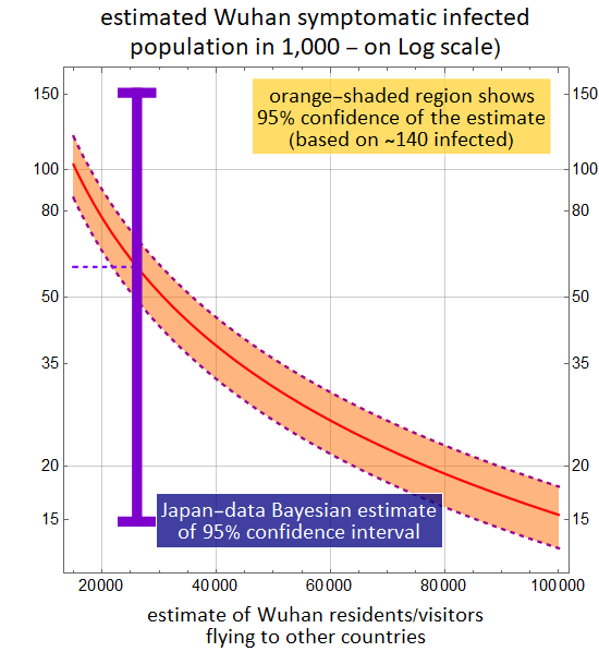
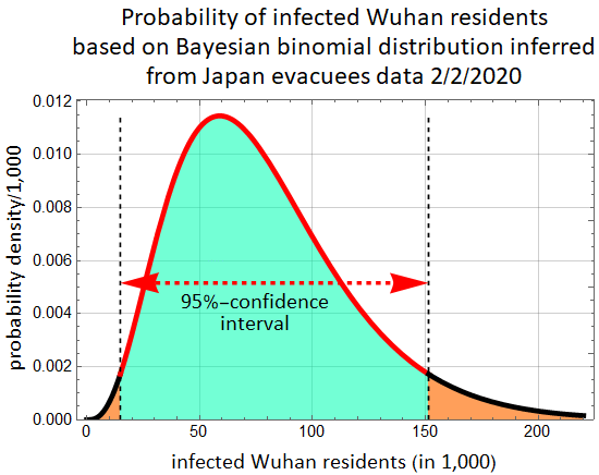
Below shows the 95%-confidence estimate of the range of symptomatic infected Wuhan residents as a function of the number of Wuhan residents/visitors flying out of China, which include the ~140 known cases of infection. There is one minor data set from Japan: 3 Japanese nationals are infected among 560 who were repatriated from Wuhan. The low-sample-population statistics of Japan data doesn't allow precise estimate, but it covers the entire range of reasonable estimates of flyer population from such a large city over a couple-week period. (e. g. 14 days with few thousand international destinations per day).

Out[48]=

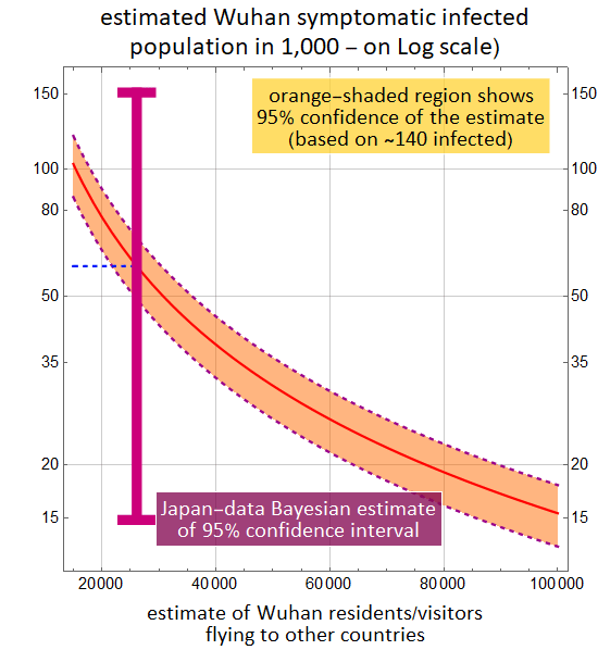
Note that as of 2/2/2020, the reported cases in all of China is just below 15,000, which is at the very low-end of all estimates. At the high-end estimate, the infected population can reach 100,000. If the silent carriers (those infected without symptoms) is 1 - 2 times of those with symptoms, the net infected population can reach several 100,000.

Out[130]=

Conclusion, it is likely that the actual number of cases in Wuhan is substantially higher than the figure of 14,400 as of 2/2/2020.

0. Overview

This is an example for us to learn about Binomial Distribution and practicing computer simulation. The topic is a part of our Lecture Topic 10: Stochastic Phenomena, Probability, Monte Carlo Methods, (although we will not get as in-depth into binomial distribution as normal distribution and Poisson distribution, since the latters are more important to us).

1. Introduction

1.1 Overall situation

Consider this: We have a population, some with infection BUT asymptomatic, and among them, some with definitive symptoms. We wish to build a model for this.

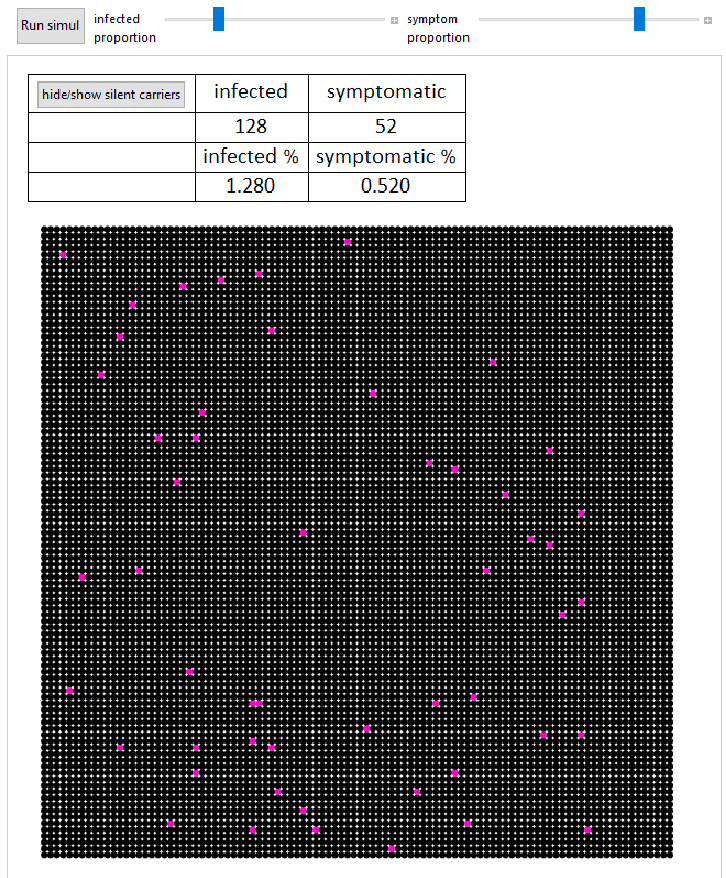
For example, below is a simulation of 10,000 dots, the symptomatic % is 0.52%. For now, it is just a number for simulation. If we imagine each dot represents 1,100 people, then it is a model of 11 million people (the population of Wuhan), and 52*1100 = 57,000 Wu-han residents exhibit the symptoms, and a larger fraction are silent carriers, not yet show any symptom.

The key data we need to simulate is the proportion of people with symptoms who left Wuhan to other countries.

Although there are reported number of cases of Wuhan-origin people who flew out of China, e. g. ~120-140 people in other countries, there has been no report of the total number of Wuhan residents on the flights. Based on the estimate number of daily international flights out of such a large and international city like Wuhan, and with an estimate of 250 - 400 passengers per flight, we can guess that ~120-140 people may represent anywhere from 0.1 to 1%.

A most definitive data is that “Three Japanese nationals among more than 560” evacuated from Wuhan have the disease. This represents a number of 0.54% that is inline with the 0.1 - 1 % guesstimate window.

1.2 Problem description

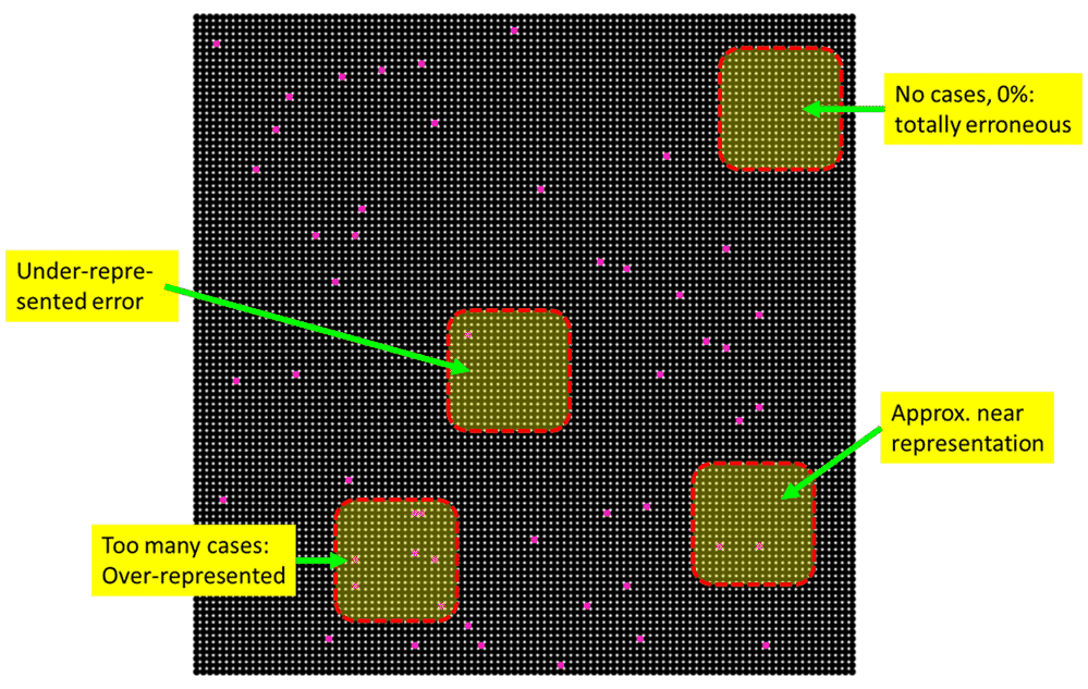
Below illustrates a well-known concept of a statistical problem: when we take a small sample out of a large population with a Bernouilly process, the estimate of the proportion can be very inaccurate, a vexing problem in social science, especially for surveying/polling social issues or political decisions (elections).

More importantly, this area of statistical science is essential in business and commerce, or customer-analytics when a company like Amazon, Google, or Facebook tries its best to estimate the probability of a particular ad would generate a pageview click or a sale with the customers.

In this case, there is another layer of estimation. A number of people who are virus carriers and vectors (an agent that carries and transmits infectious disease) have not developed the sympton, aren’t aware of their status, and are not tested. These are silent carriers.

We can define the proprotion of silent carriers (fraction of people that are infected) as p, and let ρ be the proportion of those infected with symptoms. Then, given a propulation N (e. g. the population of Wuhan),
the infected population is:   p N
the symptomatic population is  ρ p N

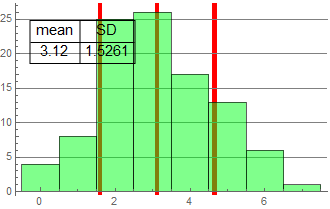
Below is the output of the same simulation model as the above, but the silent carriers are now shown as yellow dots:

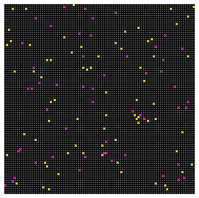
Here, it is optimistically assume that ρ=40%, in other words, for every person who exhibits symptoms, there are 2.5 total individuals infected, and not counting the one exhibits symptoms, there are 1.5 other infected individuals who don’t. With a model, we can vary these parameters.

What do we want to learn out of this? We will learn how to use Binomial Distribution theory with Bayesian inference to estimate what the symptomatic population is and what the total infected population is of Wuhan.

4. Bernouilly & binomial model for the 2019-nCoV case

Consider this: We have a population, some with infection BUT asymptomatic, shown as yellow dots, and among them, sone with definitive symptoms shown as magenta dots. We use Bernouilly distribution to simulate.

4.1 Graphics illustration with Bernouilly model

Code

Out[5]=

4.2 Consideration on estimating Bernouilly probability

There are two methods of obtaining the Bernouilly probability
                                            q = p ρ
where    p: the Bernouilly probability to be infected for a given population (Wuhan), and
              ρ: the Bernouilly probability for an infected person (the p-population above) to exhibit obvious symptoms.
In the future, if everyone suspected is tested even without symptoms, and assuming that the test has high accuracy, then, only p is relevant and one needs not be concerned with ρ. However, for the time being, q is the only parameter with measurements.

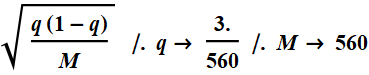
If we take as an example, 3 Japanese out of 560 flown out of Wuhan exhibited illness, then:

In[7]:=

Out[7]=

Or:                                         q=0.54%.

Immediately, we can apply binomial distribution to this sample alone, and infer that the standard of deviation (see binomial distribution lecture) of this estimate is:    

In[8]:=

Out[8]=

Or, we can write:                q=0.0054 ±0.003

However, we can attempt to include all other cases outside China. According to 2/2/2020 WHO Situation Report-13

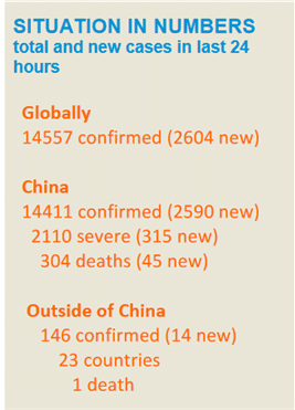
Let’s assume that of 146 cases outside China, a few are local transmission, and the rest are Wuhan fomer residents flying out of China or after visiting Wuhan, let’s round it up ~140. As a function of all Wuhan residents/visitors:

In[61]:=

Out[72]=

The essence of this is that regardless the EXACT number of total Wuhan residents/visitors who flew out of Wuhan to other countries, the range of the 95%-confidence estimate is tight number because of reasonable population statistics (10s of thousand). This means that as soon as the the actual number of Wuhan resid/visit is available, one can get a decent estimate of symptomatic infection rate q.

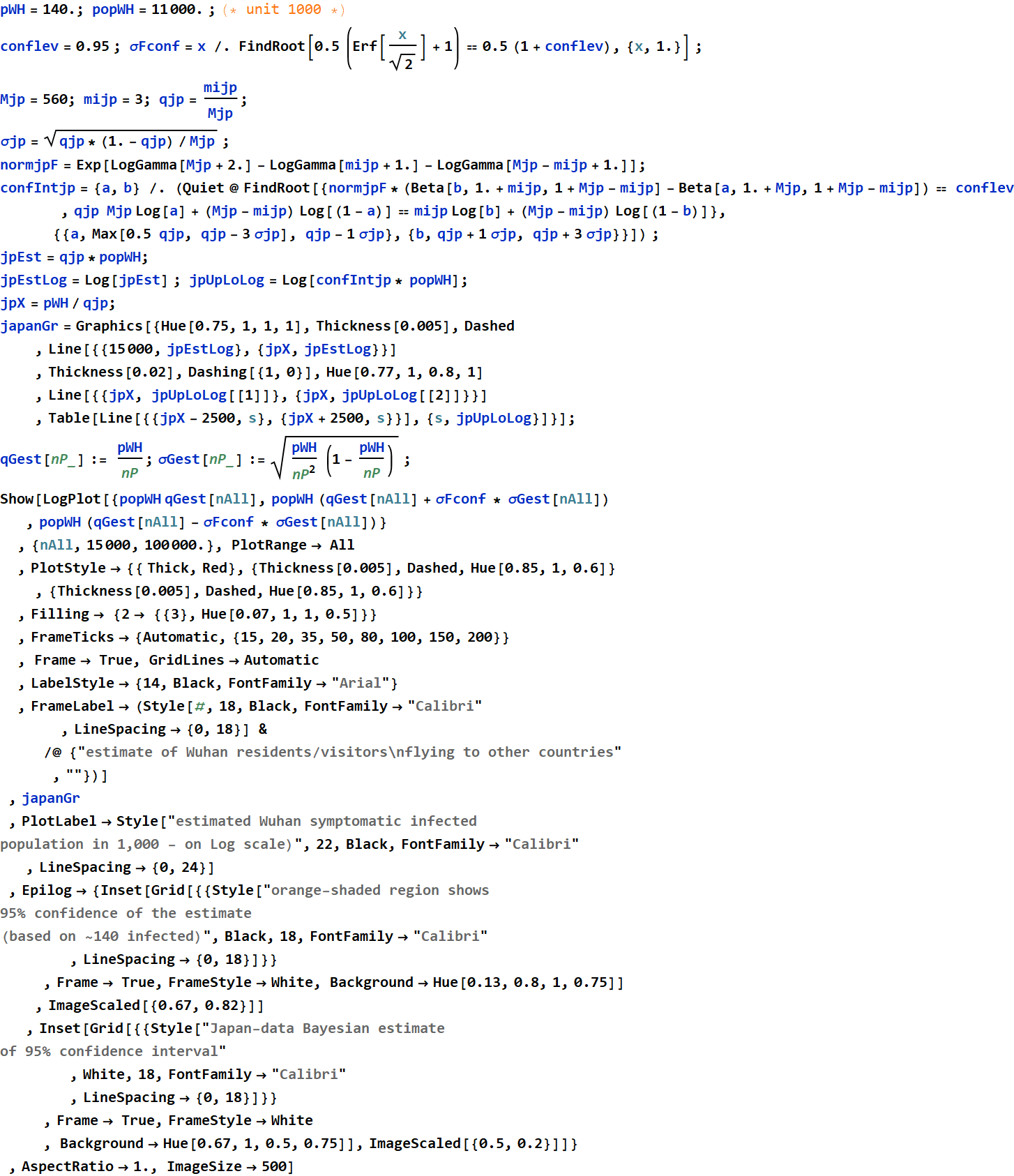
4.3 Modeling of infected population with Bayesian binomial distribution based on Japan data

There are two common methods of using the measured Bernouilly proportion to obtain a binomial model: maximum likelyhood and Bayesian. Here, we will choose only the Bayesian method. Both actually converge together with large sampled population.

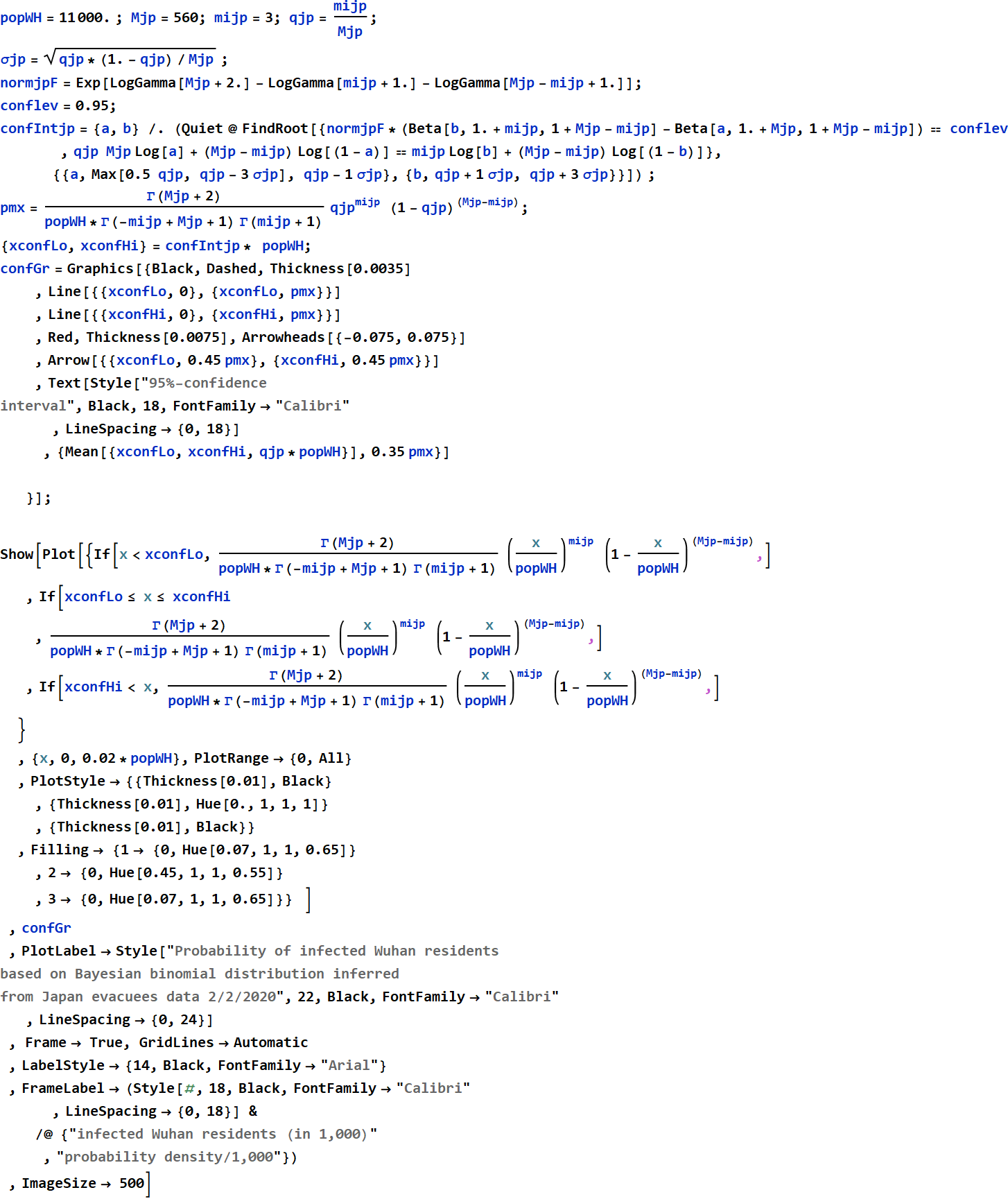
The plot for Japan data is based on the following:
            
where:              M=560 (evacuees);
The 95% confidence interval is determined as
where:                  
                       

The numerical values of the interval boundaries are:

In[131]:=

Out[131]=

which is between 0.135%  to 1.38%

In[122]:=

Out[130]=

2. Background: Categorical Variable (excerpted from Lecture) - no need to read for this case, but for reference.

Skip to Section 4 to see calculation.

2.1 A quick primer/review

Consider a typical financial statement below:

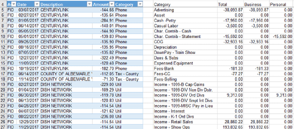
Each colum is a variable. “Date” and “Amount” are obviously numerical variables, the variables of which the values are numbers. Same are “Total”, “Business” and “Personal”. But other columns are not, they have “categories” as the entries. It is just as important to know what “category” that money is associated with. Remove those columns with categories, we would be clueless what the various amounts are for. Hence, categorical data are just as important as numerical. A lot of so-called “personalized financial analysis” done by banks are just to group or classify various monetary quantities into categories.

But not just finance, almost everything else not science and engineering involves “categorical” data as the norm.

Let’s take a look at the dataset that we have worked on before known as Credit below:

This dataset has 11 variables (not counting the 1st column, which is just the record count index). For the 1st 6 variables (columns 2-7), the variables are numerical, having continuous real values (integers are a subset of real numbers, unless used to code for categories). For columns 8-11, the variables have values that are categories, or we say they are categorical.

Variable “gender” (column 8) has only 2 values, which are categorical and not numerical. Of course we can make it numerical by assigning “female”-> 0 and “male” -> 1. But that is NOT fundamentally numerical. We can just as arbitrarily assign values: “female”-> 3.14.159 and “male” ->2.7183. In other words, assigning numerical values to a categorical variable DOESNOT make it numerical. It is only for convenience but does not change the nature of the variable.

Besides “gender”, the same are for “student status” and “marial status”, both have values “Yes” or “No”. Variable “ethnicity” has three categories as shown.

2.2 Subtypes “ordinal” and “nominal”

In general, a variable can have as many categories as needed, such as credit score (shown are 5 values, from “very poor” to “exceptional”)

This is an example showing that a numerical, continuous real-value variable can be converted into a categorical type just by choice, such as the above: the credit score is assigned into one of 5 categories.

A simple exercise

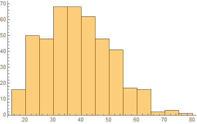
Consider another simple example. Suppose we want to collect the age data of online customers. If we collect everyone’s actual age, we will have continuous real-value data. We may have a distribution of the values as shown below:

In[2]:=

Out[3]=

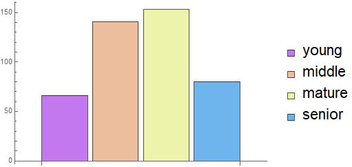
But sometimes, there is no need for the actual continuous values, because it is sufficient to group customers into age range. For example, we may need to know only whether a customer is: under 25 (young), between 25-37 (middle), or 38-50 (mature), or older (senior). Then, instead of a histogram as above, we have the statistics of categories:

In[13]:=

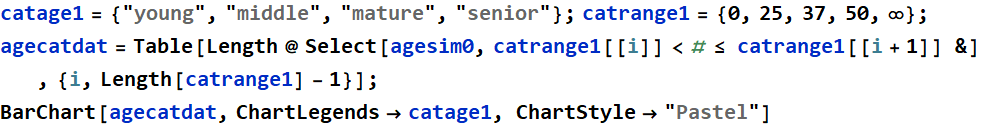
Out[15]=

One of a main reason for converting a continuous value variable into categorical type is often for the sake of simplification. Driver insurance premium, for example is computed based on one’s age group like credit score.

Consider the credit score again. Although each client has a continuous real-value credit score, e. g. 752, the only thing that matters in the end is which category the client belongs to. Financial decision, such as loan approval and interest rate is set for each category, and all scores within the same category are essentially equivalent. Hence, it is simpler to classify clients into categories.

2.3 Common graphic presentation

So, what statistics do we use to handle categorical values? For continuous values, we have distributions such as Poisson, Normal, Laplace, LogNormal etc. For category, all we have is % or fraction (* in common literature, another term for this is “proportion”, however, here, we will use the term fraction, the reason will be explained later below), for example:

In[16]:=

Out[17]=

Earlier, we learned that if we can model a continuous variable with a known distribution (e. g.Gaussian, or Laplace, or Poisson, etc. ), we can obtain the relevant parameters such as mean, SD, of β coef...  to do a model fit.

The question is, for discrete/categorical data, what do we do to simulate a distribution based on the data? The answer is Bernouilly distribution. Consider the example below.

3. Bernouilly process and binomial distribution demo - for quick review only

Skip to Section 4 to see calculation.

3.1 Basics

If you have been through previous lessons involving Bernouilly and Binomial distribution, below is a summary. If you wish more details, go to Lecture 4.

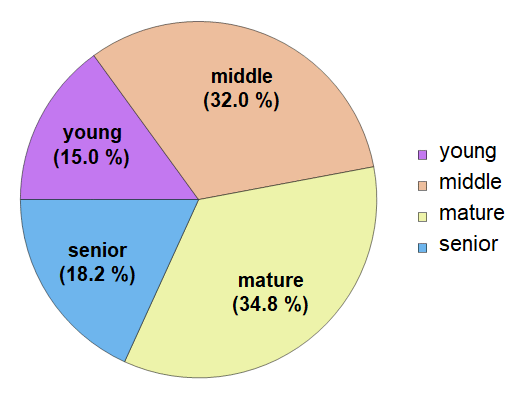
Suppose we flip a fair coin, the chance is 50-50 for head and tail. The outcome is said to have Bernouilly distribution with probability ρ=0.5. Roll a dice, the outcome of a specific number has Bernouilly distribution with ρ=1/6. Bernouilly distribution is can be a general concept for all discrete-outcome events. Recall previous examples involving roulette:

Any bet in the roulette payoff table above is an outcome that can be simulated with Bernouilly distribution.

Let’s consider a very simple example that we will use through out this note. Suppose a store near a university campus wants to monitor their customers’ profiles. First, the store wants to know how many of their customers are students so that they can develop a promotion/discount policy. After 10,000 customers, we notice 30% are students. Then, we say that there is 0.3 chance for a customer to be a student, and 0.7 chance to be non-student.
We can model the customer category like this:
- student: BD with ρ=0.3
- non-student: BD with ρ=0.7

Consider a group of 10 customers, how many of them are students, how many are not? This is a simple simulation:

In[9]:=

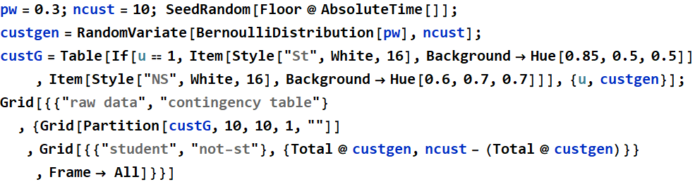
Out[12]=

Run it several times, we see that the proportion of non-stud to student is NOT always 7-3. There are statistical fluctuations as expected. Now consider 1000 customers, divided into 100 groups of 10 each, what is the number of students in each group? This is the same principle as flipping a fair coin. If we flip the coin 10 times, we can expect 5H, 5T on the average, but that does not always happen on every try. We can have 7H, 3T for one try, and 4H, 6T the next. What are the statistical properties of this randomness? Let’s examine a bit more elaborate simulation as below.

In[13]:=

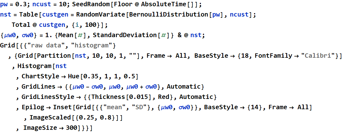
Out[16]=

raw data	histogram
1 1 1 2 4 4 0 3 2 2 3 3 1 3 5 3 2 3 7 4 4 1 4 4 4 3 2 3 1 5 3 4 4 2 2 4 3 4 4 2 3 2 4 4 1 6 2 4 3 1 3 1 3 5 3 2 3 2 4 2 5 3 1 1 4 1 3 3 2 5 2 2 3 4 4 3 3 4 3 5 4 1 3 1 3 5 2 5 3 1 4 3 3 4 4 3 4 2 3 2

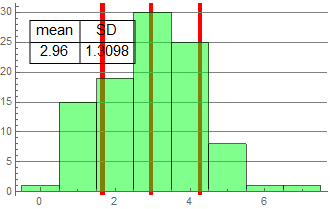
We see that while the mean of all groups is very close to the expected value of 3, there is significant deviation and the SD is large.

Another way to present it is to scale with respect to the population, which is the “percentage” or fraction: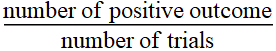
As a side note, the statistics term is “proportion” - for example, if 30% customers of a store are students, we will say the proportion of students is 0.3. However, most people always refer this quantity as “percentage” even if we don’t really express in terms of 
“percent,” i. e. 30%. People would ask “how many percents are students or what is the student fraction?”. It is OK to use whichever term that one is most comfortable with, but when we do computer simulation, the mathematical operation is to take “fraction”, Hence, we will use fraction or proportion interchangeably.

In[32]:=

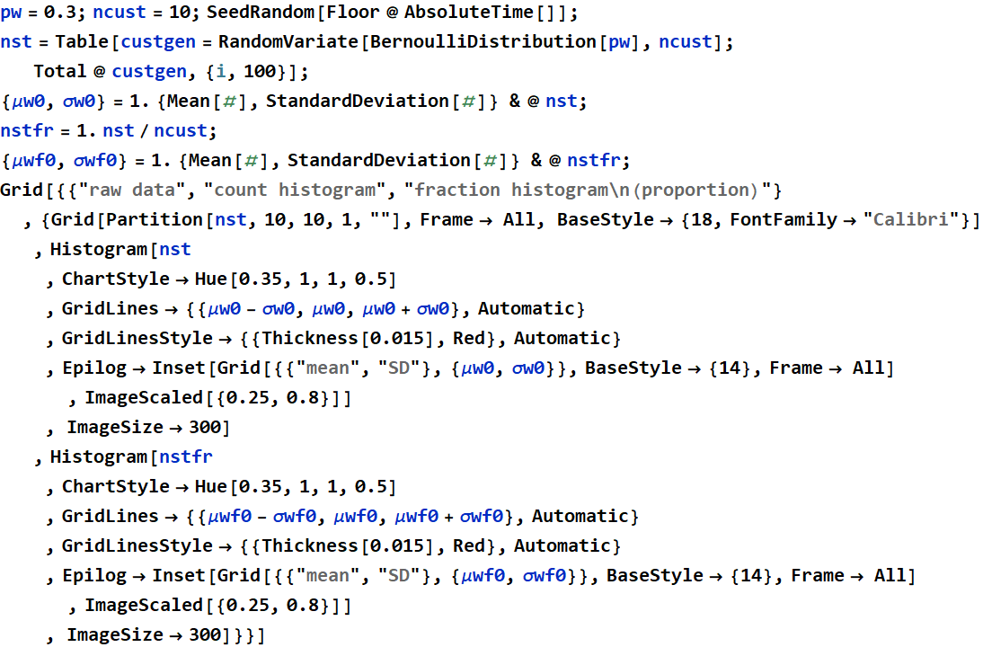
Out[37]=

raw data	count histogram	fraction histogram (proportion)
3 3 3 3 3 4 2 3 5 5 4 3 4 2 5 1 2 3 4 3 3 3 4 3 0 2 3 4 2 2 6 1 6 0 3 3 5 6 6 4 3 4 5 5 3 2 5 4 1 2 0 3 5 2 5 2 2 4 4 4 4 2 4 2 4 3 2 2 5 2 1 2 4 1 7 5 0 4 2 2 1 2 6 1 2 5 2 3 1 6 5 2 3 3 3 3 3 3 2 2

If we take larger group size, say 100 instead of 10, surely we can expect that the relative SD should be smaller. In fact, if we have ∞ number of customers, then there should not be any fluctuation, SD=0 and the mean must be exactly 0.7*∞. But what is the distribution of the above? we’ll see that it is a binomial distribution. We now can have a more elaborate simulation so that we can study this statistics.

3.2 Simulation with Bernouilly distribution outcome: binomial

Code

Out[50]=

3.3 More than two outcomes: multinouilly

What if we roll a dice, or spin a roulette? we can have more than two outcomes. We can simulate raw data similarly to Bernouilly distribution used above with a variety of techniques. Below is a convenient one:

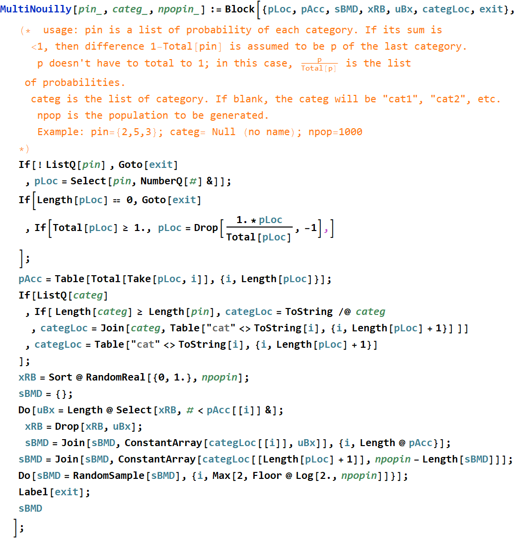
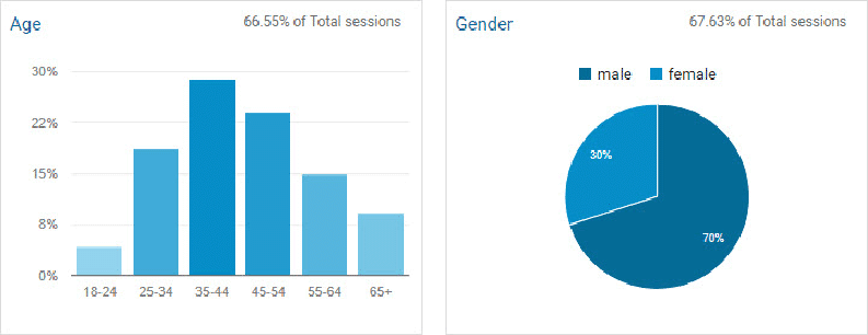
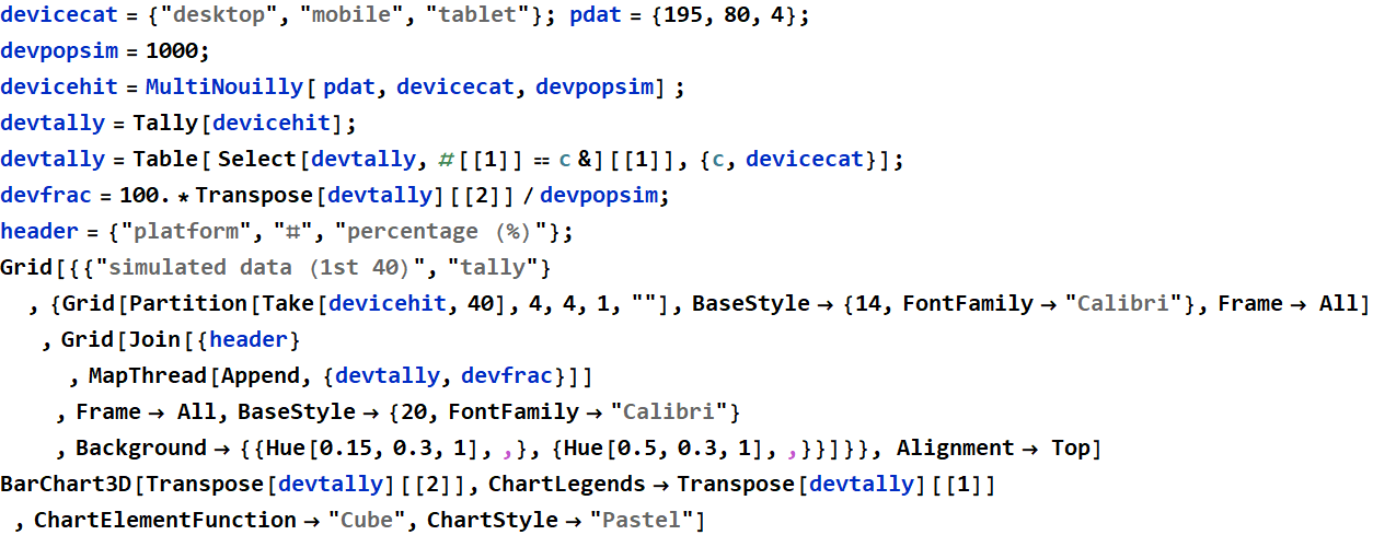
Here is an example: We want to simulate hits of a webpage. Below is the GoogleAnalytics data.

We can simulate 1000 hits based on this data (must execute the code for BernMulti above first)

In[2]:=

Out[9]=

Out[10]=

3.4 Simulation and demo of multinomial distribution

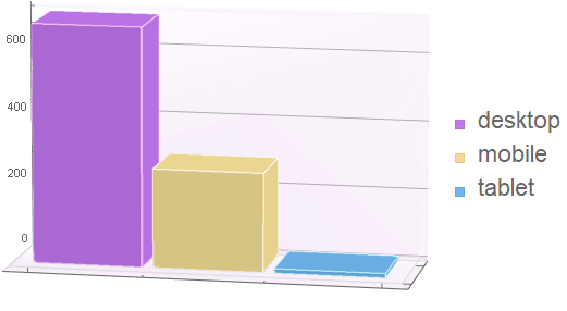
Below is an example of three main categories of user’s interests in Google Analytics. Each category has several sub-categories as shown. We will just generate a simulation for the 3 main (parent) categories: Affinity, In-Market, and Other.

Code

Out[33]=

2019-nCoV RNA