Fourier Tutorial Series - 3
Programming practicals with numerical Fourier transform

ECE 3340  & generic                         Han Q. Le (c)

It is one thing to understand the ideas and concepts, and another (totally another) thing to be able to sit in front of a keyboard and generate results - correct ones, that is.

1. Signal, carrier, and noise

1.1 A binary digital message

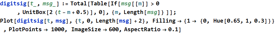
Consider we have this message:

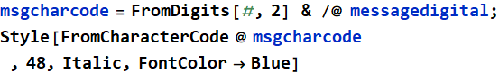
In[1]:=

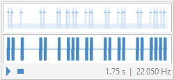
Use the bit time (1/bit rate) as a unit time, we can plot the message digitial code:

In[2]:=

Out[3]=

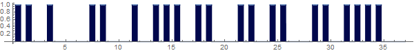
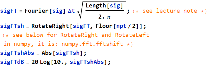
Assume a sampling rate of 8 points per unit time (duration of a bit), can we use DFT to plot the digital signal spectrum?

Approach

In[4]:=

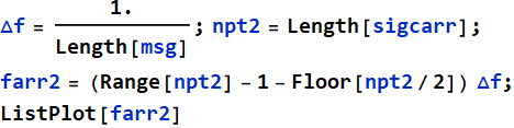
Set up the frequency array of Fourier transform:

In[8]:=

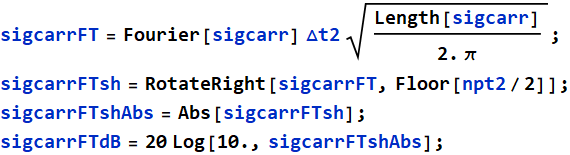
Now we do DFT:

In[11]:=

In[15]:=

In[16]:=

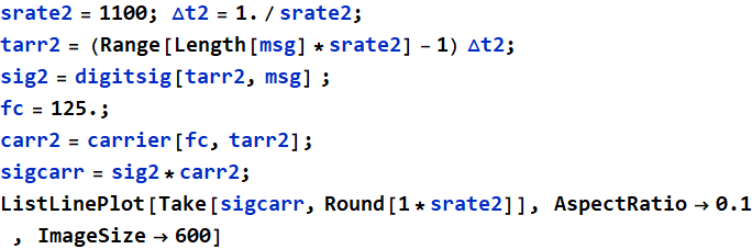
1.2 Signal with carrier

Now we use a carrier with frequency fc=125, using direct amplitude modulation. Obviously, we cannot use the same sampling rate. Here, we select sampling rate 1100 and obtain the same spectra as above

Approach

The signal function now is a product of the original signal and the carrier:

In[15]:=

We have to redefine the parameters.

In[16]:=

The signal is NOT meant for sound. It can be EM wave, but for fun, we can try make it like a sound and listen to it.

In[25]:=

Out[25]=

In[23]:=

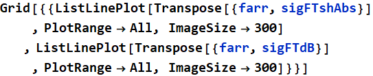
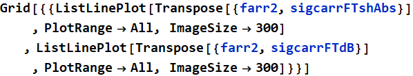
Now for FT:

In[26]:=

In[33]:=

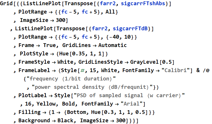
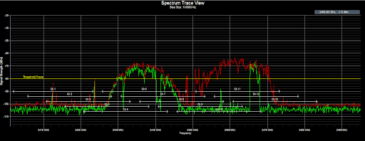
FYI, compare this to a typical wifi spectrum, except that wifi uses frequency hopping and there are no sharp single-frequency carrier lines.

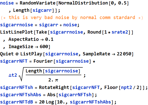
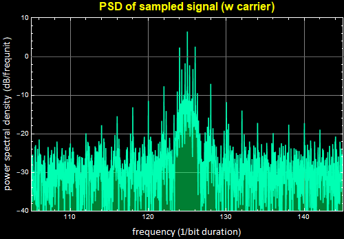
1.3 Signal with carrier + noise

We generate white Gaussian noise of amplitude 1/2 of the signal and add to the signal and obtain the spectrum again.

Approach

In[30]:=

Out[33]=

In[42]:=

If we want to filter the signal above, how wide the bandwidth should we take? Too big a BW will just add noise, but too narrow a BW will result in clipping the signal itself. What should we do? The fundamental criterion is bit-error-rate (BER), it is chosen such that the BER is a minimum. It is a stochastic problem that we will learn later in the course.

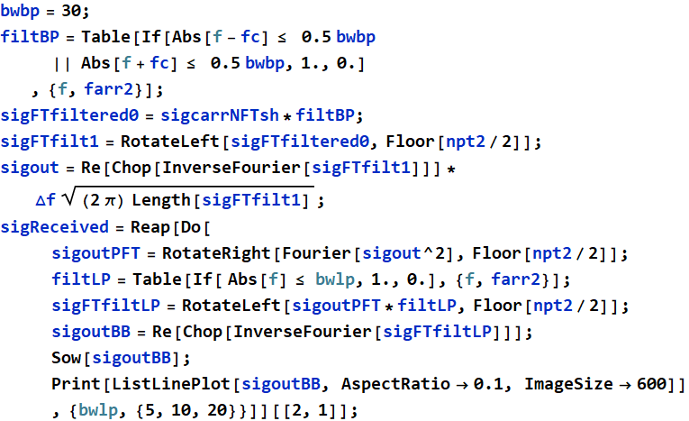
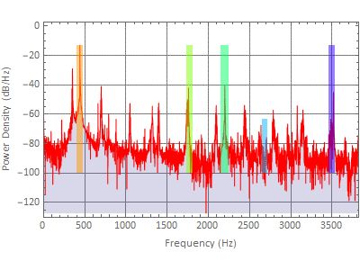
1.4 Band-pass filter

The two spectra, original baseband and with carrier & noise from the above are shown together in one plot below.

Out[162]=

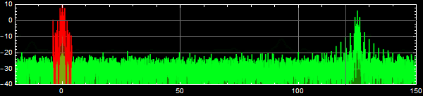
Why don’t we communicate in baseband (the frequency range in red), but always use a carrier band (such as 2.4 GHz for wifi, or Bluetooth, or RF, HF, UHF for radio and TV)? There are many reasons, one of which is that - of course, EM waves can travel much farther than any other natural waves that we know of. But interference and noise are also canonical reasons. Below are example of EM spectra in typical environment.
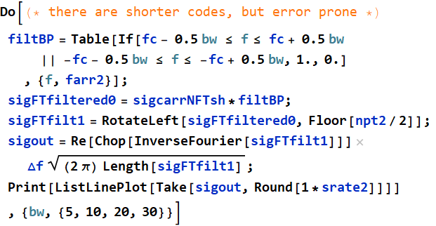
To receive our signal, it is best to use a bandpass filter: a filter that allows only the small range of frequencies around the carrier frequency. The width of the frequency range is known as bandwidth (BW or bw).
We now apply a Dirichlet filter around fc for various bw, then calculate and plot the signal output.

Approach

We will try bw=5, 10, 20, 30.

In[39]:=

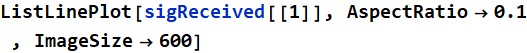
1.5 Remove the carrier

The carrier can be removed by mixing (heterodyne), since we are learning Fourier filter, we will apply that again for fun. We will use power detection (square of the signal) and then use a low pass filter to filter out the original signal, removing the carrier.
Let the signal above be filtered with a BP filter with BW=30, which is the last of the output above. Then square the output signal just like it would be with power detector, then filter it again with a low pass filter. We’ll do it for a series of low-pass bandwidth: 5, 10, 20.

Approach

In[40]:=

1.6 Decoding the message

What does the original message say?

Approach

This is the received signal:

In[50]:=

Let’s use a small function to threshold the bit (decide it is 1 or zero) and get the digital message back:

In[46]:=

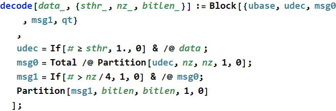
In[47]:=

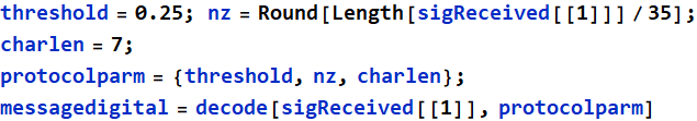
In[51]:=

2. Example: Separate two harmonic sounds

2.1 concept

Use spectrogram analysis to segment both time and frequency domain of two signals - which are two musical sounds of different pitches from two different instruments.

Instruction

We have a case of 2 or more instruments mix-up, can you separate the sound of each? A sound file of two instruments and two notes in .wav format is posted online. Alternatively, if you generate your own example that contains two different notes with two instruments, you will get 20 points bonus.
(below is an example, not the actual one posted as a .wav file)

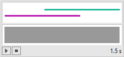
The two sounds overlap in time for 0.5 sec. Use the time before and after they overlap to determine the spectrum of each sound, and apply your filter to separate them out into two sounds.

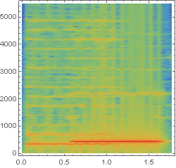
2.2 solution

Here is the spectrogram

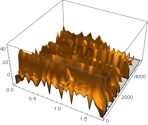Let’s zoom in:

Out[71]=

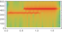
The approach is to find each sound spectrum without interference, then design filters to get each sound for the whole duration.

Analyze spectrum of first note.

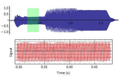
Once we select spectral filter, extend to the whole note (1 sec duration) (see spectrogram analysis). There are 11 harmonics above the noise, and we can use up to 11 narrow bands.

Above shows only 5 lines, but for a full spectrum, 11 are needed.

This is the output of 1st note: Sound 1

Do the same thing for second note:

Final answer: both notes are separated.

3. Example: image processing

3.1 Consider this example

In[58]:=

Add annotation:

In[59]:=

3.2 Fourier of Fourier:

What happens if we Fourier an object twice? i. e. Fourier of Fourier?

Out[30]=

Approach

In[60]:=

Do Fourier once:

In[62]:=

We can take a look what the Fourier spectrum is like, but remember that it has no meaning other than just to let us visualize the Fourier coefficients:

In[63]:=

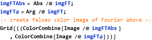
Now Fourier imgFT one more time, chop the insignificant imaginary numerical residuals, and combine them together. Put the original next to the twice-Fouriered to compare. Use this:

In[66]:=

4. Example: more advanced sound processing

Filtering of human voice from strong harmonic interference background. This involves heavier programming.

4.1 concept

Use spectrogram analysis to segment time, filter out complex human voice from interference background.

In[32]:=

In[34]:=

Out[34]=

4.2 solution

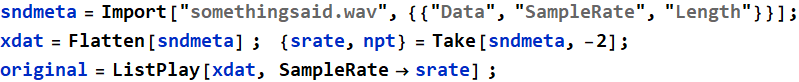
self-contained data

In[46]:=

Out[52]=

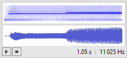
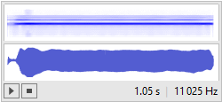
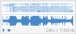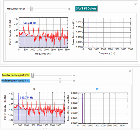
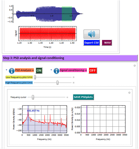
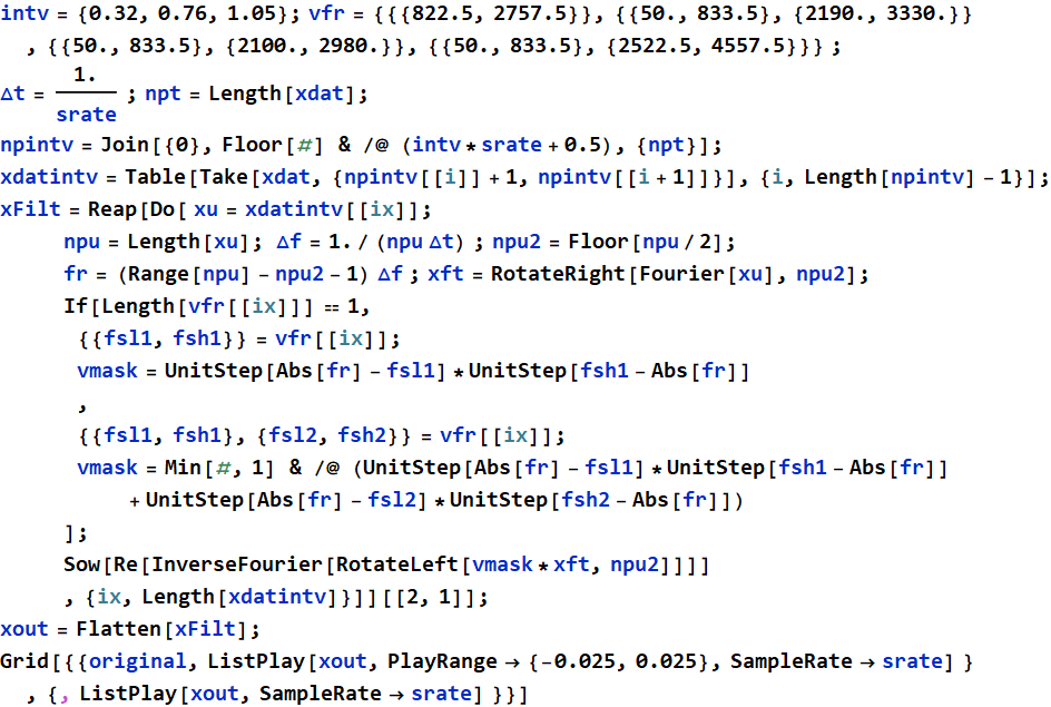
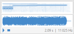
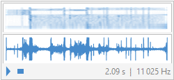
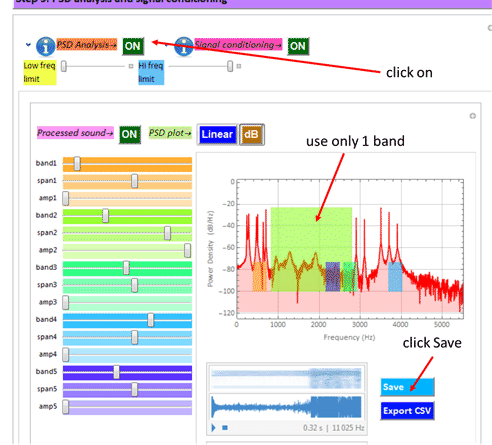
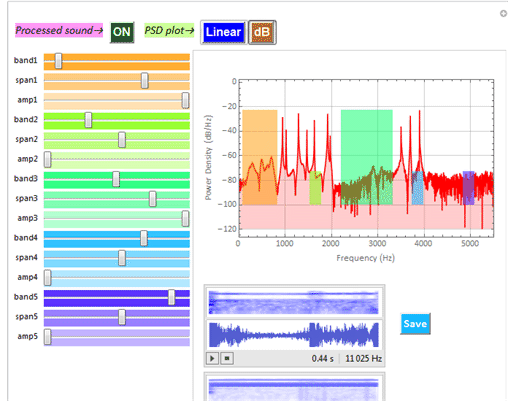
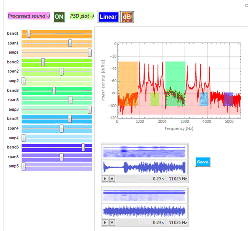
4.3 details

The background interference is not constant over the whole 2 sec, but appears to have multiple sections. Use algorithm to detect spectrogram (PSD vs time) transition to demark sections. For your convenience, here are the 4 sections:
- section 1: 0- 0.32 sec
- section 2: 0.32 - 0.76 sec
- section 3: 0.76 - 1.05 sec
- section 4: 1.05 - 2 sec
You have to process each section separately, save the results, and put all together at the end.

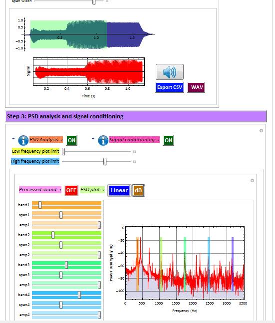
To start:

Import ,wav file, then turn on step 2 (don’t bother selecting anything), and 3 (click twice) so that the analysis stays on.

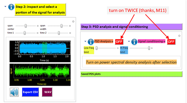
Now, analyze section one by one:

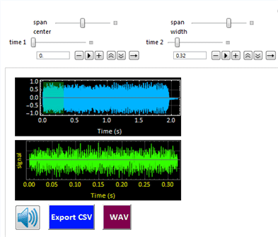
Use sliders time1 and time2 by entering the number - DO NOT HIT ENTER, just type and click somewhere else on the APP window (not on any slider) for the values to be entered.
Below is how to select section 1, from 0 - 0.32 second.

Then:

Section 1: 0 - 0.32 sec. You select the band as shown.

Section 2: 0.32 - 0.76 sec: put value in time 2 first, then time1. You select the band as shown. Then save.

Section 3: 0.76 - 1.05 sec. put value in time 2 first, then time1. Do similar

Section 4: 1.05 - 2 sec. Do similar:

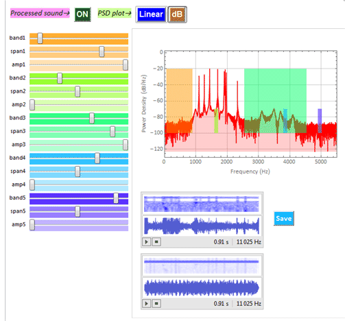
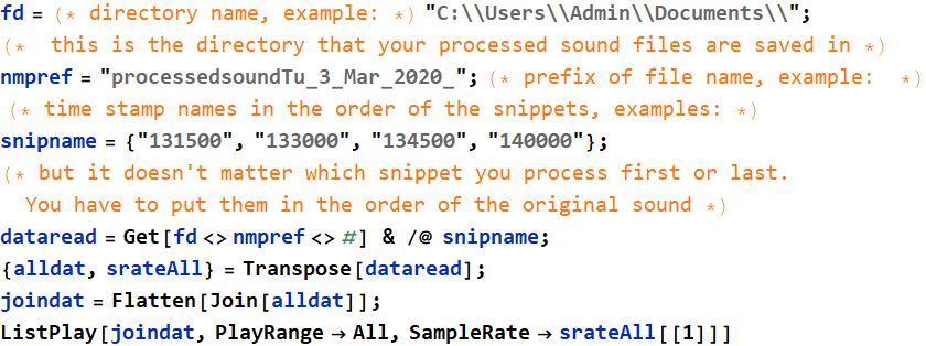
Finally, put all together :

4.4 additional code/background