Lecture 1 & 2 Numerical accuracy and precision issues

Han Q Le (c) -copyrighted

In [1]:
import numpy as np
import pandas as pd
import scipy as sp
import matplotlib.pyplot as plt

Section 1 - Floating point vs. integer

simple equation fails to hold numerically

In [5]:
x1=5; y1=np.sqrt(5);
z=x1-y1**2
In [6]:
z
Out[6]:
-8.881784197001252e-16

z is not zero as it should be: numerical error due to finite digit representation

In [7]:
np.log2(np.abs(z))
Out[7]:
-50.0

See that abs(z) is exactly 1/2**(-50)

In [10]:
print([np.abs(z), 1/(2**(50))])
[8.881784197001252e-16, 8.881784197001252e-16]

why is z exactly 2^integer? see lecture on binary representation of number in FPU Also, download related apps on apps webpage.

In [ ]:
 

consider a range of numbers

In [16]:
u1=np.array([[x,x-(np.sqrt(x))**2,np.log2(np.abs(x-(np.sqrt(x))**2))] for x in range(50)])
C:\ProgramData\Anaconda3\lib\site-packages\ipykernel_launcher.py:1: RuntimeWarning: divide by zero encountered in log2
  """Entry point for launching an IPython kernel.
In [17]:
u1
Out[17]:
array([[ 0.00000000e+00,  0.00000000e+00,            -inf],
       [ 1.00000000e+00,  0.00000000e+00,            -inf],
       [ 2.00000000e+00, -4.44089210e-16, -5.10000000e+01],
       [ 3.00000000e+00,  4.44089210e-16, -5.10000000e+01],
       [ 4.00000000e+00,  0.00000000e+00,            -inf],
       [ 5.00000000e+00, -8.88178420e-16, -5.00000000e+01],
       [ 6.00000000e+00,  8.88178420e-16, -5.00000000e+01],
       [ 7.00000000e+00, -8.88178420e-16, -5.00000000e+01],
       [ 8.00000000e+00, -1.77635684e-15, -4.90000000e+01],
       [ 9.00000000e+00,  0.00000000e+00,            -inf],
       [ 1.00000000e+01, -1.77635684e-15, -4.90000000e+01],
       [ 1.10000000e+01,  0.00000000e+00,            -inf],
       [ 1.20000000e+01,  1.77635684e-15, -4.90000000e+01],
       [ 1.30000000e+01,  1.77635684e-15, -4.90000000e+01],
       [ 1.40000000e+01,  0.00000000e+00,            -inf],
       [ 1.50000000e+01, -1.77635684e-15, -4.90000000e+01],
       [ 1.60000000e+01,  0.00000000e+00,            -inf],
       [ 1.70000000e+01,  0.00000000e+00,            -inf],
       [ 1.80000000e+01,  3.55271368e-15, -4.80000000e+01],
       [ 1.90000000e+01, -3.55271368e-15, -4.80000000e+01],
       [ 2.00000000e+01, -3.55271368e-15, -4.80000000e+01],
       [ 2.10000000e+01,  0.00000000e+00,            -inf],
       [ 2.20000000e+01,  0.00000000e+00,            -inf],
       [ 2.30000000e+01,  3.55271368e-15, -4.80000000e+01],
       [ 2.40000000e+01,  3.55271368e-15, -4.80000000e+01],
       [ 2.50000000e+01,  0.00000000e+00,            -inf],
       [ 2.60000000e+01,  3.55271368e-15, -4.80000000e+01],
       [ 2.70000000e+01,  0.00000000e+00,            -inf],
       [ 2.80000000e+01, -3.55271368e-15, -4.80000000e+01],
       [ 2.90000000e+01,  3.55271368e-15, -4.80000000e+01],
       [ 3.00000000e+01,  0.00000000e+00,            -inf],
       [ 3.10000000e+01,  3.55271368e-15, -4.80000000e+01],
       [ 3.20000000e+01, -7.10542736e-15, -4.70000000e+01],
       [ 3.30000000e+01,  0.00000000e+00,            -inf],
       [ 3.40000000e+01,  0.00000000e+00,            -inf],
       [ 3.50000000e+01,  0.00000000e+00,            -inf],
       [ 3.60000000e+01,  0.00000000e+00,            -inf],
       [ 3.70000000e+01,  7.10542736e-15, -4.70000000e+01],
       [ 3.80000000e+01,  7.10542736e-15, -4.70000000e+01],
       [ 3.90000000e+01,  0.00000000e+00,            -inf],
       [ 4.00000000e+01, -7.10542736e-15, -4.70000000e+01],
       [ 4.10000000e+01,  0.00000000e+00,            -inf],
       [ 4.20000000e+01,  0.00000000e+00,            -inf],
       [ 4.30000000e+01,  7.10542736e-15, -4.70000000e+01],
       [ 4.40000000e+01,  0.00000000e+00,            -inf],
       [ 4.50000000e+01, -7.10542736e-15, -4.70000000e+01],
       [ 4.60000000e+01,  0.00000000e+00,            -inf],
       [ 4.70000000e+01,  0.00000000e+00,            -inf],
       [ 4.80000000e+01,  7.10542736e-15, -4.70000000e+01],
       [ 4.90000000e+01,  0.00000000e+00,            -inf]])
In [22]:
x1arr=u1[:,0]; z=np.abs(u1[:,1]);
plt.plot(x1arr,z)
Out[22]:
[<matplotlib.lines.Line2D at 0x1a4729f3438>]

create a range from 0 to 1,000,000

In [24]:
u2=np.array([[x,x-(np.sqrt(x))**2,np.log2(np.abs(x-(np.sqrt(x))**2))]
             for x in np.arange(0,1000000,2503)])
x2arr=u2[:,0]; z2=np.abs(u2[:,1]);
plt.loglog(x2arr,z2)
C:\ProgramData\Anaconda3\lib\site-packages\ipykernel_launcher.py:2: RuntimeWarning: divide by zero encountered in log2
  
Out[24]:
[<matplotlib.lines.Line2D at 0x1a472b84400>]

Note that the error grows proportionally with th number magnitude: this is because the same error in the mantissa is multiplied with the exponent: intrinsic error in the mantissa

Section 2 - sinusoidal error with large argument

Consider this problem
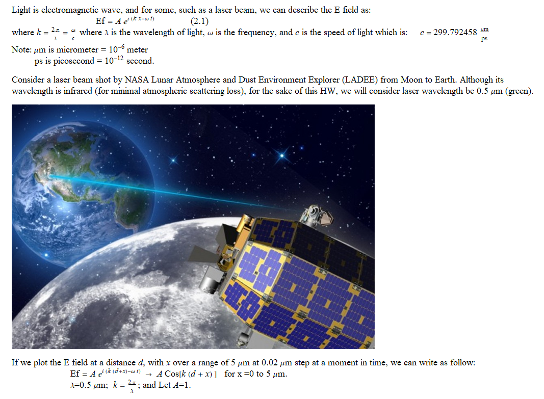
plot EM wave at d=0

In [26]:
wl=0.5; k=2*np.pi/wl ;   xarr2=np.arange(0,5,0.02);
d=0;
ef1=np.cos(k*(d+xarr2))
plt.plot(xarr2,ef1)
Out[26]:
[<matplotlib.lines.Line2D at 0x1a47475a7b8>]

plot EM wave at d=384000 km

In [27]:
wl=0.5; k=2*np.pi/wl ;   xarr2=np.arange(0,5,0.02);
d=384000e9;
ef3=np.cos(k*(d+xarr2))
plt.plot(xarr2,ef3)
Out[27]:
[<matplotlib.lines.Line2D at 0x1a4747ba278>]

for d=1000 km, error is small, but can be seen

In [30]:
wl=0.5; k=2*np.pi/wl ;   xarr2=np.arange(0,5,0.02);
d=1000e9;
ef2=np.cos(k*(d+xarr2))
plt.plot(xarr2,ef2)
Out[30]:
[<matplotlib.lines.Line2D at 0x1a4748db898>]

Plot the difference between ef2 and ef1, we can already see loss-of-precision numerical error

In [31]:
plt.plot(xarr2,ef1-ef2)
Out[31]:
[<matplotlib.lines.Line2D at 0x1a4736acdd8>]

The numerical error of cosine grows with argument magnitude. The correct way is to use the periodic property of the function:

In [36]:
wl=0.5; k=2*np.pi/wl ;   xarr2=np.arange(0,5,0.02);
d=384000e9;d0=np.fmod(d,wl);
efcorrect=np.cos(k*(d0+xarr2))
plt.plot(xarr2, efcorrect, 'g', xarr2, ef3, 'r')
Out[36]:
[<matplotlib.lines.Line2D at 0x1a4749d8898>,
 <matplotlib.lines.Line2D at 0x1a4749d89e8>]

Similar errors

In [37]:
x=np.arange(-1,1,0.05)
sinx=np.array([np.sin(2*np.pi*2*n*1000 + x*1.e-11) for n in range(1,4)])
plt.plot(x,x*1.e-11,'b')
[plt.plot(x,sinx[i],'r') for i in range(len(sinx))]
Out[37]:
[[<matplotlib.lines.Line2D at 0x244419f0748>],
 [<matplotlib.lines.Line2D at 0x24441a90ba8>],
 [<matplotlib.lines.Line2D at 0x24441a90ef0>]]

The plot below is Sin[n 2 Pi +x] vs x where n is an integer. The result should be a straight line (blue) because: Sin[n 2 Pi +x] = Sin[x] ~ x for small x (which is on the order of 10^-11). Yet for large n, ~ few 2000, one can see errors due to loss of precision as well as biases due to a large argument.

System epsilon, largest, smallest

small number add to large number

In [4]:
epsilon=0.123456789e-14
In [5]:
epsilon
Out[5]:
1.23456789e-15
In [11]:
y=1+epsilon 
delta=y-1
print([delta, epsilon])
[1.3322676295501878e-15, 1.23456789e-15]
In [19]:
x=np.arange(-1,1,0.0125); xeps=x*1e-15 
y=1+xeps
plt.plot(x,y-1,'r',x,xeps,'b')
Out[19]:
[<matplotlib.lines.Line2D at 0x1abf82a62e8>,
 <matplotlib.lines.Line2D at 0x1abf82a6438>]

largest number and smallest number

In [33]:
x=np.arange(0,2,0.5)*1e308
np.array([x,2*x])
C:\ProgramData\Anaconda3\lib\site-packages\ipykernel_launcher.py:2: RuntimeWarning: overflow encountered in multiply
  
Out[33]:
array([[0.0e+000, 5.0e+307, 1.0e+308, 1.5e+308],
       [0.0e+000, 1.0e+308,      inf,      inf]])

soft (or slow) flush to zero

In [44]:
x=1e-322
for  i in range(6):
    x=0.5*x
    print(x)
5e-323
2.5e-323
1e-323
5e-324
0.0
0.0
In [ ]: