Class blog 3/5

ECE 3340 - Han Q. Le (c)

Additional notes and HW4A

See this tutorial for the main help on HW4A

1. Details of Problem 1B

Since some indicated interest in prob 1B of HW 4A. Here are the details that you should do:

Detailed specification: (this is included in the revised HW 4A)

1. The noise standard deviation, which is the term σ in
RandomVariate[LaplaceDistribution[0.,σ],Length[x]]
must be >= 2 times the rms of your signal. In other words:

2. The interference must have 10 times xrms:

where fint is your choice between 1500 to 2000 Hz.

See Class blog 3/5 for details of the rest.

Other things you need

Use spectrogram to separate the sound snippets. Example: for this recording (replace with your own):

it is OK for you to use it without noise and interference to obtain a clean spectrogram so that you can get the time intervals.

Here is to get the spectrogram:

Obtain the spectrogram:

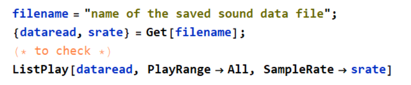
First, get the data:

Then:

Out[598]=

Use the spectrogram for time interval separation

Use the spectrogram, or analyze the original recording in anyway you wish, but only for time interval separation, such as for "I", "am", "Ro", "bert".
Example : soundwave and this spectrogram shows :
   "I" : t = 0.1 - 0.305 s;
   "am" : 0.305 - 0.38;
   "Ro" : 0.38 - 0.585;
   "bert" : 0.585 - 0.75

Perform spectral filtering for each snippet

Must show and explain your filters, of course. This part is where most of your score will come from.

Assemble the snippets for final output.

After getting all the snippets:

2. Additional things you can do for Prob. 3

2.1 You can plot the Fourier spectrum before and after the filter

Example: This is BEFORE filtering

In[618]:=

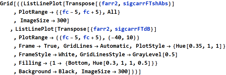
Out[618]=

this is after the filtering:

In[637]:=

2.2 You can plot or listen to the signal before and after filtering

This is the noisy signal:

In[638]:=

Out[638]=

In[639]:=

Out[639]=

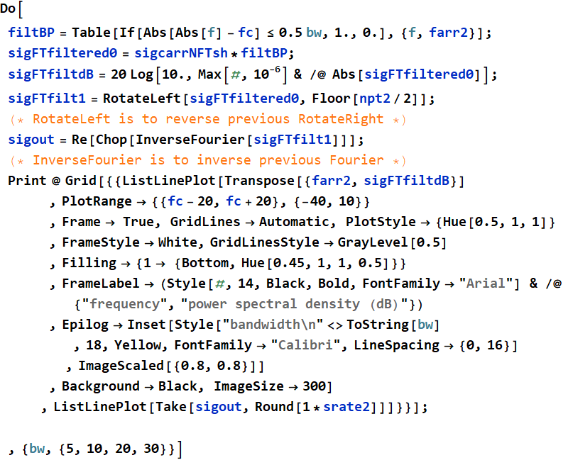
After filtering with bandpass filter with bandwidth = 30: (Don't forget to discuss the difference: this is the whole point about filtering the signal & carrier band out of a broad spectrum with white noise distribution).

In[640]:=

Out[647]=

Out[648]=

One important note about the App

After filtering each sound or snippet, and after listening to make sure that it is what you want, click blue-background "save" button beneath the spectrum plot, you will see it prints the name of the file that the sound output is saved to.
Below is an example (see the long file name at the bottom).


however, you will not see it in .wav or .mp3: it is in raw number format for Mathematica only. Then follow the instruction how to obtain the data array after you close the app. Below is the simplest:


One annoying thing with Mathematica version 10 and up is that it will restart the dynamic loop several times to re-initialize the variables each time we open a new function. It means that the PSD Analysis button will go off a couple times before staying ON as shown below. Just re-click the ON button when it goes OFF. It needs to stay ON to connect the data from DataSelect window to the data in Signal Conditioning window. Once the selected data are correct, you can disconnect the two windows by using the unlink icon button at the top of the Signal Conditioning window.

Make sure to reconnect again when you select a different part of the sound. One way to verify is to always check with the plot in the PSD Analysis window as shown below. Click "Signal conditioning" button OFF, you will see the PSD of the selected signal. Click the "Signal conditioning" button on, the PSD graph is off, but you should see the equivalent PSD graph is the Signal Conditioning window. This feature was developed when Math 10 replacing Math 9. It crashed repeatedly if both charts are on. It might be OK with Math 12 now, but better safe than sorry because Mathematica graphics FrontEnd has a lot of issues ever since after Math 9.





On another note: When you enter direct data:
ALWAYS enter a single-dimensional array of number. If you record a sound in the stereo mode, you will have two channels. Simply use [[1]] to select only channel 1 (or [[2]] for channel 2). But only one channel will be processed. You can enter this way: {mysound[[1]], srate} or {mysound[[2]],srate}