ECE3340 Numerical Methods |
|
|||
Class blog 2/14
ECE 3340 - Han Q. Le (c)
Questions from the class and things for next week.
1. Questions
1.1 How did you figure out the numbers in the array coef that will ...create the heart-shape?
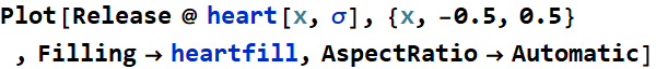
Start from drawing the heart shape with an analytic formula (see CW)
In[1]:=
In[3]:=
Out[3]=
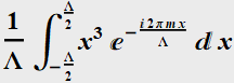
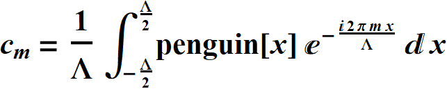
Then, the
coefficients are simply obtained by the Fourier
theorem:
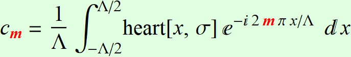
where Λ is the period.
The code was given explicitly:
In[8]:=
Out[10]=
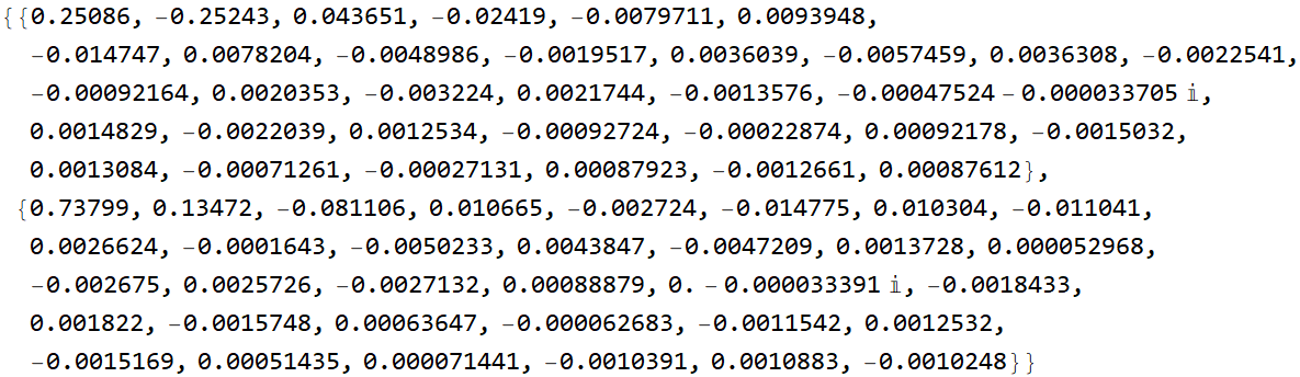
The above are the coefficients (trimmed to 4 digits) and given in the classwork assignment.
1. 2 How did you know that using Cos function will create the heart-shape, instead of using Sin function, or Tan function, or Sec function?
ONLY SIN or COS functions form the complete ORTHOGONAL basis for the Fourier theorem. TAN and SEC are NOT the basis functions (see more in Section 2). This is critical.
Why only using Cos and not Sine?
Fourier theorem states:
Then, take the complex conjugate:
Since f[x] is
real: ![]()
Hence: 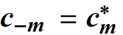
Thus we can add pair-wise:
![]()
This is the reason we write:
Re[ coef .
fExpn ] in the code.
Special case: Even or symmetric
function: f[-x]
= f[x]
then: ![]()
Hence: ![]()
Thus, we can use only Cos and no
need for Sine.
The other special case: Odd
or anti-symmetric function: f[-x]
= -f[x]
Then: ![]()
It follows:
Since: 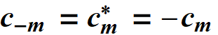
![]() must be purely
imaginary:
must be purely
imaginary: ![]()
and the
product ![]() is
real as expected.
is
real as expected.
Example of this case of odd function was when we did in the class for an odd function:
In[35]:=
Out[35]=

Substitute
In[36]:=

Substitute again:
In[37]:=
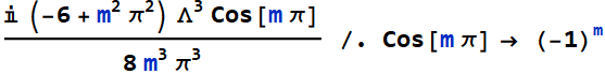
Out[37]=
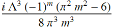
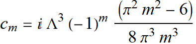 is
a purely imaginary quantity.
is
a purely imaginary quantity.
The answer: because heart-shape function is an even function, hence, we can use only Cos functions, and they are sufficient. But never ever think of Tan or Sec as the basis functions for the Fourier series - please see Section 2.
1.3 How did you know that taking the dot product of coef and fcosn will create 2 arrays that when you plot, you will get the heart-shape?
See answer in 1.1 above. The coefficients were taken by the formula for Fourier series coefficients, hence what we do is simply reconstruct the original, up to the frequency that we choose (32 in this case).
Here is something to look at again to understand:
To draw a penguin, we need 12 single-value functions (12 drawing lines) as shown below. Beside 12 functions, we also need two constant lines for coloring. Execute to understand:
In[11]:=
This is the plot of penguin function:
In[18]:=
Out[20]=
We can get the Fourier coefficients by simply
apply:
These lines of code do it:
imgFourier=fouriergraphics2[{funcname,σ,
styleparm},nchan,nintv];
Here is the explanation how it is done inside Block
function fouriergraphics2
Read through the code below to understand the steps involved.
In[25]:=
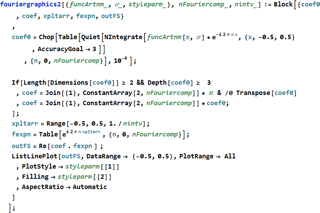
The output of the above function is to reconstruct - or to do a Fourier synthesis of the function that we input, which, in this case, is penguin function.
In[30]:=

Out[33]=
 |
 |
Out[34]=
| time taken: | 16.024110.656318859285346 | sec. |
If we use only 3 Fourier components: m=1, 2, 3, this is how it looks:
In[40]:=

Out[43]=
 |
 |
Out[44]=
| time taken: | 1.234696.5431048789768385 | sec. |
If we use only 4 Fourier component: m=1, 2, 3, 4, this is how it looks:
In[35]:=
Out[38]=
 |
 |
Out[39]=
| time taken: | 1.523922.634507783521069 | sec. |
1.4 For example, if I want to plot a chair-shape, where should I begin with? How can I figure out the method?
Write a multi-value function to describe the chair the same way as penguin function describes a penguin, then do this: change funcname to chair with appropriate filling color for the chair.
![]()

That’s it.
Here, this is a simple example of the half-moon bridge:
In[45]:=

This is how it looks:
In[48]:=
Out[49]=
Now, see this:
Out[63]=
 |
 |
Have fun! I suggest drawing a recliner. But here are more interesting artworks that had been tried by other students in the past. They didn’t look exactly the same. I only recalled the ideas.
 ,
, 


Just a few as examples. It was given as HW, but too
labor-intensive for most, only a fraction of the class could do
it. Triangle function (for pine tree) and Ellipse function (for
penguin) were given. Students just combined them such as the witch
hat, or ice cream cone.
2. Dot product in Fourier series theorem
2.1 Formal review (if you forgot linear algebra)
In an N-dimensional space with basis vectors:
![]()
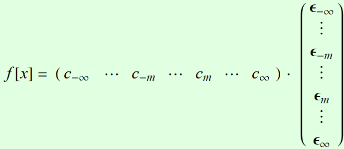
Any point (or element) in that space can be
represented as a DOT product:
One can use the transpose format of the above, which is fine.
In Fourier
series theorem, the functions:
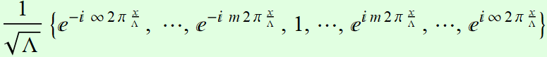
form a complete
orthonormal basis system: (infinite-dimension space) like
the u basis vectors
above.
For those who care about formal mathematics, the vector space in
this case is the space of
piece-wise continuous, square-integrable functions,
defined in a finite interval. For convenience, we can let that
interval be [0, Λ).
Then. the inner product of two vectors (i. e. two functions) f[x]
and g[x] is
defined to be:
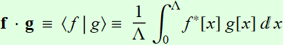
(Notation bra <
| and ket |
> are very useful in physics).
Denoting the
function 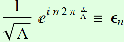
Then, the set
![]() for
for ![]()
forms a complete
orthonormal basis system:
The above is equivalent with: ![]() that are often used for the linear space of
that are often used for the linear space of ![]()
Hence, any
piece-wise continuous, square-integrable function f[x]
in that interval can be represented as:
Or:
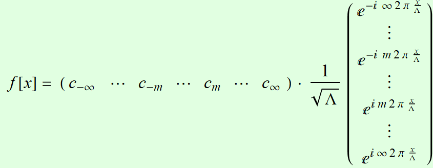
which is (in
conjugate-pair-wise arrangement)
For a real-value function, there is no need to add the negative
index part, we only need the positive index part and take the real
part of the whole expression.
2.2 Formalism vs. numerical implementation with coding
The first
commandment (or professional imperative) of numerical methods:
Thou shall do correct
calculations.
The proof-of-the-pudding of understanding and practical skill is NOT about reproducing formulas or proofs. It’s about the capability to code to generate correct numerical results.
In our computer
coding, it is:
![]()
![]()
Hence: outFS=Re[coef . fexpn ] ;
and that
is why we use dot product.
Remember:
Fourier functions are not only the basis functions of the space of piece-wise continuous,
square-integrable functions, of course. We can
arbitrarily generate an infinite number of basis systems simply
using a linear transformation:
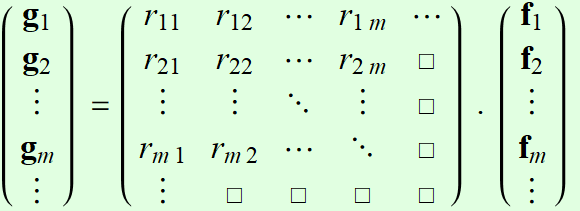
where R transformation
martrix must be invertible or has non-zero determinant.
Numerous systems of basis functions are important in physics and
engineering. Legendre, Laguerre, Hermite, Chevbyshev...
polynomials are all well known. Other functions such as Bessels
with Fourier azimuthal ![]() ,
and Associated Laguerre polynomilas with spherical harmonics are
important for differential equations of 2nd order in cylindrical
and spherical coordinate.
,
and Associated Laguerre polynomilas with spherical harmonics are
important for differential equations of 2nd order in cylindrical
and spherical coordinate.
2.3 True/proof-in-the-pudding skills: correct coding.
2.3.1 Example 1:
If you don’t feel comfortable with
formal mathematics above, it is OK, just learn how to express in
code correctly for numerical calculation. Follow this recipe:
1- IF THE COEF ARE GIVEN, then:
2- IF YOU WANT TO FIND THE COEF, then:
Example: half circle:
In[32]:=
Out[33]=
In[64]:=
Out[66]=
| 0.392699 +0. i | 0.0711538 +6.07153*10^^-18 i | -0.0265478-2.81893*10^^-18 i | 0.0147271 -8.67362*10^^-18 i |
| -0.00965818+8.67362*10^^-19 i | 0.00695125 -4.33681*10^^-18 i | -0.0053087-5.20417*10^^-18 i | 0.00422459 +0. i |
| -0.00346506-2.60209*10^^-18 i |
See the meaningless residuals in ![]() ?
To clean them up:
?
To clean them up:
In[71]:=
Out[74]=
| 0.392699 | 0.0711538 | -0.0265478 | 0.0147271 |
| -0.00965818 | 0.00695125 | -0.0053087 | 0.00422459 |
| -0.00346506 |
There is no need to integrate with so much accuracy and precision:
In[75]:=
Out[78]=
| 0.392699 | 0.0711535 | -0.0265527 | 0.0147313 |
| -0.00966308 | 0.00695548 | -0.00531361 | 0.0042288 |
| -0.00346995 |
FYI, function like half-circle has exact analytic results:
Out[89]=

It involves Bessel
function J: 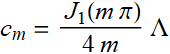
Bessel functions are known as the Sine, Cos, and Exp of the
cylindrical coordinate.
But here, we use pure numerical method to handle any function (not specific like half-circle). To reconstruct, use the recipe above:
In[100]:=
Out[104]=
2.3.2 Example 2:
Remember that a function can be a mapping from R to ![]() ,
in other words, a scalar can be mapped to a vector in
N-dimensional space. Below, is a 3-values function:
,
in other words, a scalar can be mapped to a vector in
N-dimensional space. Below, is a 3-values function:
Try to apply the above and see what you get. You will learn the important skill of array handling when having to deal with multi-value function.
Use this for the output:
Answer (only if you get stuck)
3. Things for next class(es): Fourier from space to time
The objective in the next two lectures is to get to the concept of Fourier transform, and then learn discrete Fourier transform for numerical Fourier analysis. We also make a major transition: we study Fourier theorem for applications with space, now we will study it for applications with time.
From space:
to time: 
3.1 Review basic concepts of time periodic signals
Physical concepts of time periodic signals: see app below
Out[2]=
Review the mathematica object we use to describe the above physical signal: Euler’s complex number notation and for circuit, we call it phasor.
 |
 |
![]()
Although the signal can be described with harmonic functions sine or cosine in the Real Number space R, it is more fundamental as well as mathematically more efficient to describe periodic phenomena in the Complex space C
3.2 Fourier synthesis: generate a time signal
We will continue to do Fourier synthesis, but not for drawing. The variable in Section 1 above is x, which is for physical space, used for visual rendering of images. This time we will apply Fourier synthesis to time, variable t.
![]()
Instead of space period Λ, we deal with time period T, and the
most important parameter in this case is:
frequency  unit:
unit:
 , if
, if
![]() , it is Hz
, it is Hz
or: angular
frequency ω=2 π f unit:
 such as radian
Hz.
such as radian
Hz.
Remember that in the complex plane, ![]() is a rotating point (or vector). It is the mathematical model for
virtually all wave phenomena in nature. In circuit, we use this
math for phasor. Learn more by downloading apps or visit the part
on phasor in other courses.
is a rotating point (or vector). It is the mathematical model for
virtually all wave phenomena in nature. In circuit, we use this
math for phasor. Learn more by downloading apps or visit the part
on phasor in other courses.
Note also that we drop ![]() :
it is a meaningless constant in time-varying signals that we are
interested in. Hence, set it as 0.
:
it is a meaningless constant in time-varying signals that we are
interested in. Hence, set it as 0.
3.3 Numerical approach: coding a function using Block or Module to generate a time signal
Suppose we wish to generate a time signal, what do
we need to know:
1- the frequency: call it freq
2- the amplitude and phase: this is represented as the complex
amplitude of a phasor:
![]()
3- the sampling rate: how often do we sample the signal as output?
t is continuous, but there is no such a thing as a continuous
numerical array, we have to sample time with a finite set of
discrete sampling point. Let’s call it srate
4- duration: how long in time is the signal? The signal may be
forever, but numerically, there is a finite size of an array of
numbers to be generated.
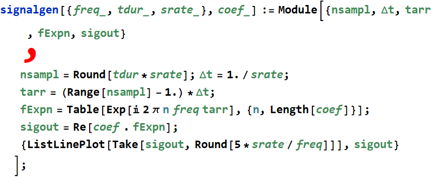
So, below is an example of such a function, we call it signalgen for signal generator:
In[11]:=
Example how to use it: we will generate a random signal:
In[26]:=
Out[32]=
End
You are strongly encouraged to go through all the tutorials up to
now. Send in questions if need help.