Tutorial 4 / CW
on Numerical Accuracy and
Precision
Treat part of this as lecture materials. You should study and practice at home.
1. ListPlot/LineLinePlot practice
Plot Cos[x] for x from 0 to 50 by making a ~500-point array. Do with an array of point instead of built-in function.
In[144]:=
![]()
Out[144]=
Answer
In[10]:=
Out[12]=
2. Problem 2 - EM wave long distance
Light is electromagnetic wave, and for some, such
as a laser beam, we can describe the E field as:
![]() (3.1)
(3.1)
where ![]() where λ is the wavelength of light, ω is the frequency, and c is the speed of light which
is:
where λ is the wavelength of light, ω is the frequency, and c is the speed of light which
is: 
Note: μm is micrometer = ![]()
ps is
picosecond = ![]() second.
second.
Consider a laser beam shot by NASA Lunar Atmosphere and Dust Environment Explorer (LADEE) from Moon to Earth. Although its wavelength is infrared (for minimal atmospheric scattering loss), for the sake of this HW, we will consider laser wavelength be 0.5 μm (green).

If we plot the E field at a distance d, with x over a range of 5 μm at
0.02 μm step at a moment in time, we can write as follow:
![]() for
x =0 to 5 μm.
for
x =0 to 5 μm.
λ=0.5
μm; ![]() ;
and Let A=1.
;
and Let A=1.
2.1 Plot E-field at source
Let d=0, plot E field.
Answer
x range is from d+0 to d+50 (μm). Efield is the cos
of that.
![]()
![]()
In[13]:=
Out[17]=

2.2 Plot E-field at d=1000 km
Plot the field after having traveled a distance d=1000 km away from its
starting position.
Note: to convert km to μm: 1 ![]() .
.
Answer
In[18]:=
Out[22]=
2.3 Plot the E field when it reaches Earth at d = 384000 km.
Plot the E field when it reaches Earth at d =
384000 km. ![]() μm)
μm)
Answer
In[23]:=
Out[27]=
2.4 Discussion
Is the above correct result? i. e. is that the electromagnetic field when it reaches Earth? Discuss.
Answer
No. Electric field as expressed
by ![]() remains
the same regardless of distance: periodic vs.
remains
the same regardless of distance: periodic vs. ![]() .
The graph is caused by a loss of accuracy
and precision in
the computation.
.
The graph is caused by a loss of accuracy
and precision in
the computation.
2.5 Is there any difference between E field after 1000 km vs E field at the starting position? They �look� the same
Is there any difference between ef2 (E field after
1000 km) with ef1 (E field at the starting position)?
Hint: plot xarr2 vs. ef2-ef1
Answer
�Look� can be deceiving. We must be aware of the error long before it becomes obvious to the eye.
In[28]:=
![]()
Out[28]=
We see that the error is already there. quite big,
~ ![]()
In[18]:=
![]()
Out[18]=
It is the same error, just that it becomes so big that it is now obvious.
Understanding (operational knowledge) of computer limits means to be aware of errors long before they become disastrous.
2.6 What is the �Numerical-Methods�-wise correct approach?
Answer
Don�t force a
function out of its computationally valid range:
![]() ,
or Sin, Cos
,
or Sin, Cos ![]() :
all of them, as performed by the FPU of your CPU, have errors
depending on the input variables.
:
all of them, as performed by the FPU of your CPU, have errors
depending on the input variables.
Here, the correct solution is to use the periodicity property:
In[29]:=
Out[33]=
Lecture break: mantissa, exponent, precision, accuracy
Goto Course Notes webpage for Lecture 2. Link here.
3. Problem 3 - numbers inside a computer
3.1 ![]() ,
find
,
find ![]()
Let x1 be some number, y1=![]() ,
find z =
,
find z =![]() .
.
Answer
3.2 Do 3.1 above with ![]()
Now, let x1=5., use computer to calculate z
In[34]:=
![]()
Answer
In[35]:=
Out[36]=
![]()
3.3 Take ![]() of z
of z
Answer
In[37]:=
![]()
Out[37]=
![]()
If ![]() ,
it means
,
it means  .
Let�s verified:
.
Let�s verified:
In[38]:=
![]()
Out[38]=
![]()
why? we�ll see that in the lecture about binary computer architecture: Lecture Set 3. Link here.

3.4 Make a Table of many numbers
Make a table (array) of {x1 (integer), z=Abs[ ![]() ], and
Log[2,z]} for x1 from 0 to 50.
], and
Log[2,z]} for x1 from 0 to 50.
Answer
In[39]:=

Out[40]=
| 0 | 0. | Indeterminate |
| 1 | 0. | Indeterminate |
| 2 | 4.44089*10^^-16 | -51. |
| 3 | 4.44089*10^^-16 | -51. |
| 4 | 0. | Indeterminate |
| 5 | 8.88178*10^^-16 | -50. |
| 6 | 8.88178*10^^-16 | -50. |
| 7 | 8.88178*10^^-16 | -50. |
| 8 | 1.77636*10^^-15 | -49. |
| 9 | 0. | Indeterminate |
| 10 | 1.77636*10^^-15 | -49. |
| 11 | 0. | Indeterminate |
| 12 | 1.77636*10^^-15 | -49. |
| 13 | 1.77636*10^^-15 | -49. |
| 14 | 0. | Indeterminate |
| 15 | 1.77636*10^^-15 | -49. |
| 16 | 0. | Indeterminate |
| 17 | 0. | Indeterminate |
| 18 | 3.55271*10^^-15 | -48. |
| 19 | 3.55271*10^^-15 | -48. |
| 20 | 3.55271*10^^-15 | -48. |
| 21 | 0. | Indeterminate |
| 22 | 0. | Indeterminate |
| 23 | 3.55271*10^^-15 | -48. |
| 24 | 3.55271*10^^-15 | -48. |
| 25 | 0. | Indeterminate |
| 26 | 3.55271*10^^-15 | -48. |
| 27 | 0. | Indeterminate |
| 28 | 3.55271*10^^-15 | -48. |
| 29 | 3.55271*10^^-15 | -48. |
| 30 | 0. | Indeterminate |
| 31 | 3.55271*10^^-15 | -48. |
| 32 | 7.10543*10^^-15 | -47. |
| 33 | 0. | Indeterminate |
| 34 | 0. | Indeterminate |
| 35 | 0. | Indeterminate |
| 36 | 0. | Indeterminate |
| 37 | 7.10543*10^^-15 | -47. |
| 38 | 7.10543*10^^-15 | -47. |
| 39 | 0. | Indeterminate |
| 40 | 7.10543*10^^-15 | -47. |
| 41 | 0. | Indeterminate |
| 42 | 0. | Indeterminate |
| 43 | 7.10543*10^^-15 | -47. |
| 44 | 0. | Indeterminate |
| 45 | 7.10543*10^^-15 | -47. |
| 46 | 0. | Indeterminate |
| 47 | 0. | Indeterminate |
| 48 | 7.10543*10^^-15 | -47. |
| 49 | 0. | Indeterminate |
| 50 | 7.10543*10^^-15 | -47. |
3.5 Obtain array {x1,z}, name it u2, and ListPlot x1 vs. z
In[41]:=
Out[42]=
3.6 Do the same as 3.5 but x1 from 0 to 1000000 in step of 2503 and use ListLogLogPlot
In[75]:=
Out[75]=
![]()
Out[77]=
Notice something: the error grows proportionally with the number magnitude: the error is in the mantissa, and it grows proportionately with the exponent.
Extra: For those who want to see an example of linear regression
In[85]:=
Out[88]=
![]()
Out[90]=
In[91]:=
![]()
Out[91]=
The power coefficient is ~1. It means the error grows linearly with respect to the number magnitude. The reason is that the number is stored as two parts: mantissa and component. Example:
Doesn�t matter how big a number is, the main change
is in the 11-bit exponent, the mantissa precision error is almost
the same (multiplied by the exponent).
Rule of thumb: Precision error is
in the 52-bit mantissa. Magnitude (out-of-range) errors such as
overflow and underflow are in the 11-bit exponent.
Lecture break: Binary, 64-bit float number - intro
Goto Course Notes webpage for Lecture 3: Binary Computer Architecture: Link here.
4. Revisit Problem 2 - EM wave
2.6 What is the �Numerical-Methods�-wise correct approach?
Answer
Don�t force a function out of its computationally
correct range:
![]() ,
or Sin, Cos
,
or Sin, Cos ![]()
Use periodicity:
why can�t we use Mod for the sum of d+xarr2? What if we do?
In[100]:=
Out[102]=
Out[103]=
This is what happens if we add a big number (d) to a much smaller (relatively) array:
In[108]:=
Out[109]=
Go to lecture and app for more details:
Lecture break: Floating-point - IEEE-754- detail
Use this app to get a feeling:
Home assignment (possibly) discussion
Consider this RC circuit:
Let the input be a square wave:
Out[16]=
The output is:
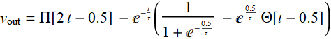 for 0≤
t < 1 (2.1)
for 0≤
t < 1 (2.1)
and is periodic with period of 1; τ is the RC time constant:
For the notation of Eq. (2.1) above:
Π[u]
is the UnitBox
function
Θ[u]
is the Heaviside UnitStep function
Below is an example of the output for τ=0.1
code
In[110]:=
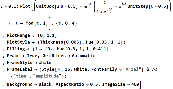
Out[110]=
1 Plot the output for τ=0.01
Answer
code
We set τ=0.01;
In[111]:=
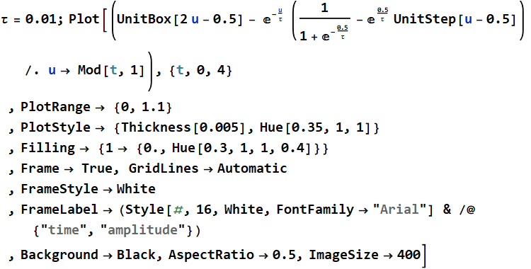
Out[111]=
2 Plot the output for ![]() ,
for t from 0.5 to 0.5005
,
for t from 0.5 to 0.5005
You must explain your approach how to get the solution.
Answer
See mini homework 2