Bonus: in Part A, Step 5, you have two options. Option B has 35% bonus.      Option A: observe demonstrations either live or recorded of the rectification experiment, write your observation, interpretation, and understanding. Recommendation: watch the recorded demonstration at your leisure and bring questions, if any, to the meeting for discussion.     Option B: if you wish, you can do some experiments on AC rectification, write a thorough report for extra credit: 35% worth of a regular lab. Please go to update pages for the latest modification, class-wise issues, and others  - Lab 2 Update page a  - Lab 2 Update page b

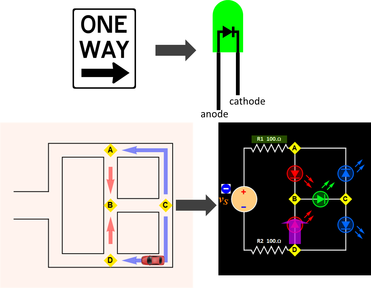
In this lab, we will try to build a circuit that represents this traffic pattern:



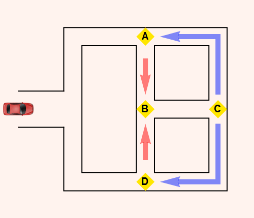
We will do this to convert one-way traffic sign into electrical one-way current flow:

Outcomes:

• You will build and study two simple circuits that are variations of the Wheatstone and rectifier bridges.

• You will perform voltage and current measurements to verify Kirchhoff's circuit laws on these circuits.
  

Objectives:

To reinforce your understanding of Kirchhoff's current law and voltage law. To gain more experience with building and measurements of circuits.

Introduction:

Consider the two circuits below. The rectifier on the left is ubiquitous in virtually all devices and appliances with AC-DC converters. It demonstrates how to control the current flow with diodes. With a load on v_out, the current is directed from the source to the load via either node A or D to node B and is returned from node C to either node D or node A. With regard to Kirchhoff's Circuit Laws, although it is a trivial case when the diode reverse current is neglected, it is an important illustration of current conservation and efficiency, as the diodes prevent the current at either node A or D from flowing onto unwanted paths.

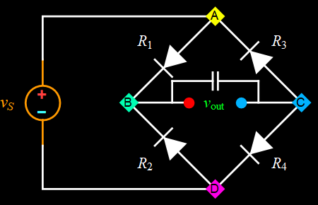
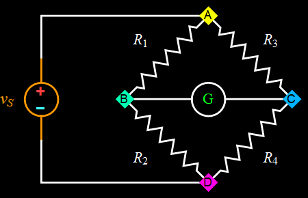
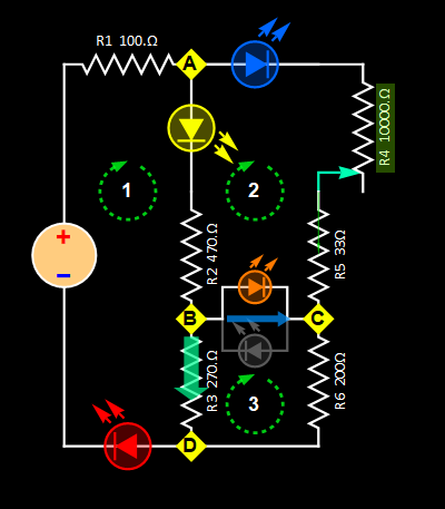
The Wheatstone bridge on the right demonstrates how to control the voltages of different nodes in a circuit. With appropriate control of the resistors, the voltages of node B and C can be made balanced with respect to each other (i. e. equal to each other), and there will be no current flow. With a current flow sensor (galvanometer G), based on the current direction, one can see which node has the higher voltage as the resistances of one or more resistors are varied. It serves as a very simple but non-trivial illustration of Kirchhoff's Circuit Laws when galvanometer G is a circuit element with finite (not infinite) impedance.

Rectifier bridge	Wheatstone bridge
Circuit 1	Circuit 2
Fig. 1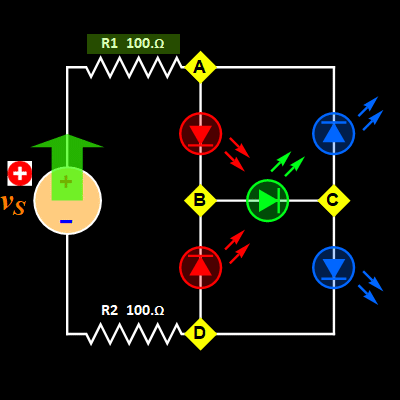	Fig. 2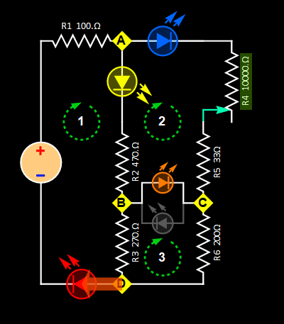

In this Lab., we will build and study Circuit 1 and Circuit 2 above, which are variations of the rectifier and Wheatstone bridges with a modern feature: LEDs are used to visualize the current flow. The objective is certainly not to build the original circuits for their utilitarian values (which would be trivial and boring). The goal of this Lab is to build advanced variation versions to enable insights and intuitive understanding of how the circuits work by reinforcing experimental measurements with direct visual experience. The essence of KCL in application is about the distribution and balance of voltages and currents. These circuits serve as simple examples to study Kirchhoff's Circuit Laws.

Background: Kirchhoff's Circuit Laws applied to the circuits

This ECE 2100 lab course is to develop your empirical learning of the circuit theories in ECE 2201 (and other circuit/signal analysis courses). Please review KCL and KVL as necessary from other courses. Here, we study Kirchhoff's Laws via experiments, but will not engage in any detailed theoretical calculation. Both Circuits 1 and 2 above have an app each to help you comparing your experimental results with calculations. Please go to appendix page i for instruction how to use the app. Below is an explanation of the algorithm in the app. It is highly desirable for you to understand, but do not be concerned for now if you don't. You can still do the lab work and run the apps without worrying about the nitty-gritty details.

1.  For Circuit 1

Since we use the zero-current reverse bias approximation for the diodes, the LED rectifier bridge is really just one-mesh circuit, albeit polarity-division-multiplexing. It is one shape of mesh for positive source voltage, and a different shape for negative source voltage. The mesh is obvious in the animated gif Fig. 1 above.

The only difference is the two pairs of LED: LED1 (AB) and LED4 (CD) for positive, and LED2 (DB) and LED3 (CA) for negative.

2. For Circuit 2
   

There are two configurations for Circuit 2: without bridge and bridged. Consider the case of without BC bridge:


There are only two meshes, the KCL equations are:


where Rvar is the sum of R4 and R5. The green terms are unknown variables to be solved for.


With a bridge between nodes B and C, which is a bidirectional LED or a pair of reverse-polarity LEDs (we consider them as the same), we have two cases as illustrated below.

Case 1: current flow from node C to B	Case 2: current flow from node B to C

Theoretically, the two cases are the same, but not for practical calculation since the bidirectional LED between nodes B and C has a  different I-V characteristic for each current direction (which is necessary for it to emit different colors). This type of LED is specifically designed to be a flow-direction indicator. A most common use of this type of LED is for two-state indication sensor such as battery charging (current flow one way) and discharging (current flow the other way). In this lab, we can just use two parallel LEDs as shown if we don't have a bidirectional LED. The KCL equations are:

Note the different subscripts (a and b) for the bidirectional LED4, which is also labeled LEDbd. Rvar is the sum of R4 and R5.
And:





Note the different subscripts (a and b) for the bidirectional LED4 (or LEDbd). Rvar is the sum of R4 and R5. The app for this circuit simply solve these equations numerically, using input resistance values and calibrated models for LEDs. Since the latter are based on the LEDs we distributed for you to use, if you use your own LEDs, their IV curves might be different and the results can be different, but should not be too much. Below are the IV models used for the app.

    

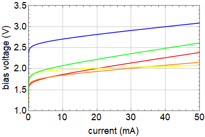
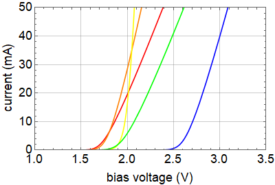
The bidirectional LED has its own calibration, and it is similar to the green and orange LED above. When we use a pair of LEDs as a substitute for bidirectional LED, we simply use the known calibration.
 

Continue to next page (2)