|
|
A further note for students who have had, or currently take Signal Analysis ECE 3337 or those who wish to look ahead to ECE 3337 At this point you have learned Laplace transform and its application to circuit transient response. This course is NOT supposed to teach you circuit theory, but only to provide laboratory support to your studies of circuits. However, it is useful to review and reinforce your learning whenever possible. The circuits for Lab 5 are extremely simple but they serve as useful examples of applications of Laplace transform technique. You are supposed to do some straight forward calculation of various RC time constants. But do you wonder how to simulate the signals on an oscilloscope? You need to solve the circuits and it is a good occasion to reinforce the learning of Laplace transform.
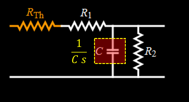
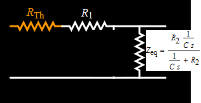
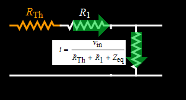
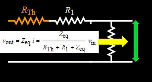
The rest is just algebra. We plug Zeq in the expression for vout (really, just tedious algebra but very simple in concept) 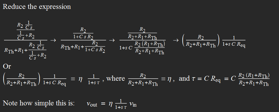 Discussion Note something here: the "R" in the RC time constant is the EQUIVALENT resistor of the parallel circuit of (R1+Rthevenin) and R2. The serial equivalence for R1 and Rthevenin is expected, because they are in series, obviously. But why is it parallel for R2 with (R1+Rthevenin)? It is because they are indeed parallel when the voltage goes to zero. The lower the load resistance R2, the quicker the capacitor discharges. The Laplace transform method shows clearly how they are connected, resulting in an effective time constant. Also, note the amplitude eta, which is the divider voltage of R2 for serial R1, R2, Rthevenin. This is also obvious, because for a given constant source voltage, R2 voltage is its divider portion for the three in series. Again the Laplace transform method gives the result in a simple and straightforward manner. Laplace transform and inverse Laplace transform Now we have to find the Laplace transform of vin, which is just a square pulse in this case. Then we have vout Laplace transform and all we have to do is to get the inverse Laplace transform of Vout to get its time function expression. The whole deal is captured in the figure below: 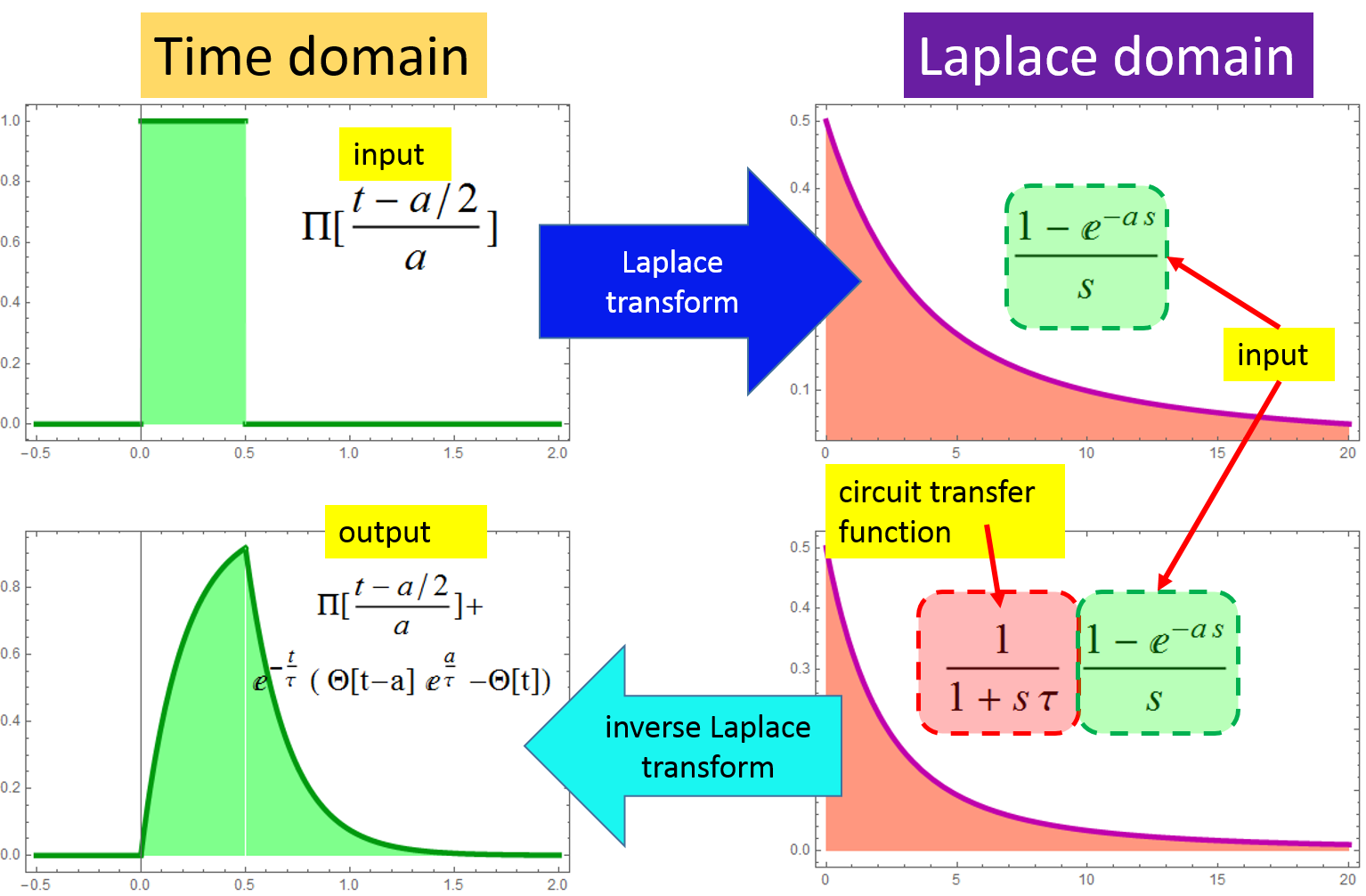 Hence:  Square wave signal The above result is just for one square pulse of duration a and RC time constant tau. We also need to simulate for square wave input. This can be done as follow. 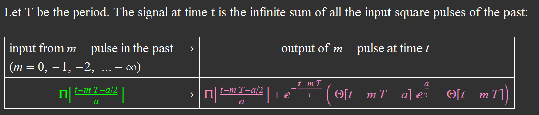 We can perform the sum as follow: 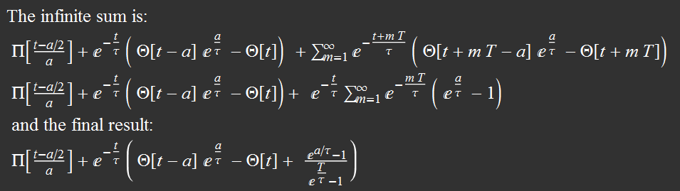 The above result is for one period t from 0 to T. Modulo function can be used to plot for any number of periods. Results for differentiation circuit We can obtain similar results for differentiation circuit. For one square pulse: 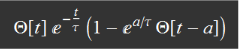 For a square wave, the function for one period t from 0 to T is: 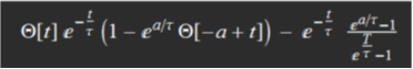 |
||||||||||||||||||||||||||||||||||