Lab work modification: TBD (after class survey and Lab 4)

 

Part A - Capacitor-enabled self-oscillatory op amp circuit


Step A.3:  Sound circuit: do not be concerned if you don't have the exact R, C components shown in wiring diagram or the simulation app. Use any pair of R C with the closest values to the recommended or default values of the app. The key point, as mentioned in the Guide, is to have it in the audio range so that you can hear. In other words, 1/RC is from 1 - 2 kHz. Then you can tune the potentiometer for higher or lower audio frequency.

Step A.4:  LED circuit. The sample principle of the Sound circuit above applies: for this, the LED flashing rate should be in the human eye time-response range.



Part B - Differentiation circuit

Step B.1: When building the circuit, use the closest components you have to the nominal values. Enter your values in the circuit simulation app  and check the results within the range of frequency of interest, ~ 100 Hz to 10 kHz. See the Guide page video for examples of results. Do not just decide on components and start doing measurements without checking, otherwise, you may waste time measuring unwanted results. See the note on frequency response and Bode plots in Step B.3 below.


Step B.2: The most basic test of differentiation (and most common in applications) is to get a constant rate of change with a ramp input. This is why we use a saw tooth or triangle wave to see a square wave. In some sensor applications, before the days of digital control with microprocessor that numerically calculates the derivative (if you are an Arduino digital PID control enthusiast, you know what this means), this is actually used for controlling the rate of change of actuator. It can be used with digital control for feedback.


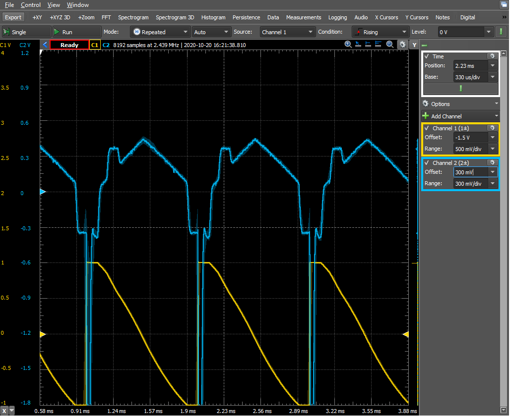
Step B.3: Below is an example of a problem with a Digilent AD2: please do not blindly submit a thing like the below ("that's what the machine did..."). It may be just a problem with this unit, or something else. For whatever reason, it is the experimenter's responsibility to ensure the veracity and quality of the data and data analysis. Digilent AD2 is just a tool. Some aspects of the tool are useful and correct, we should use them. Some are not and we must use our judgment not to use it.




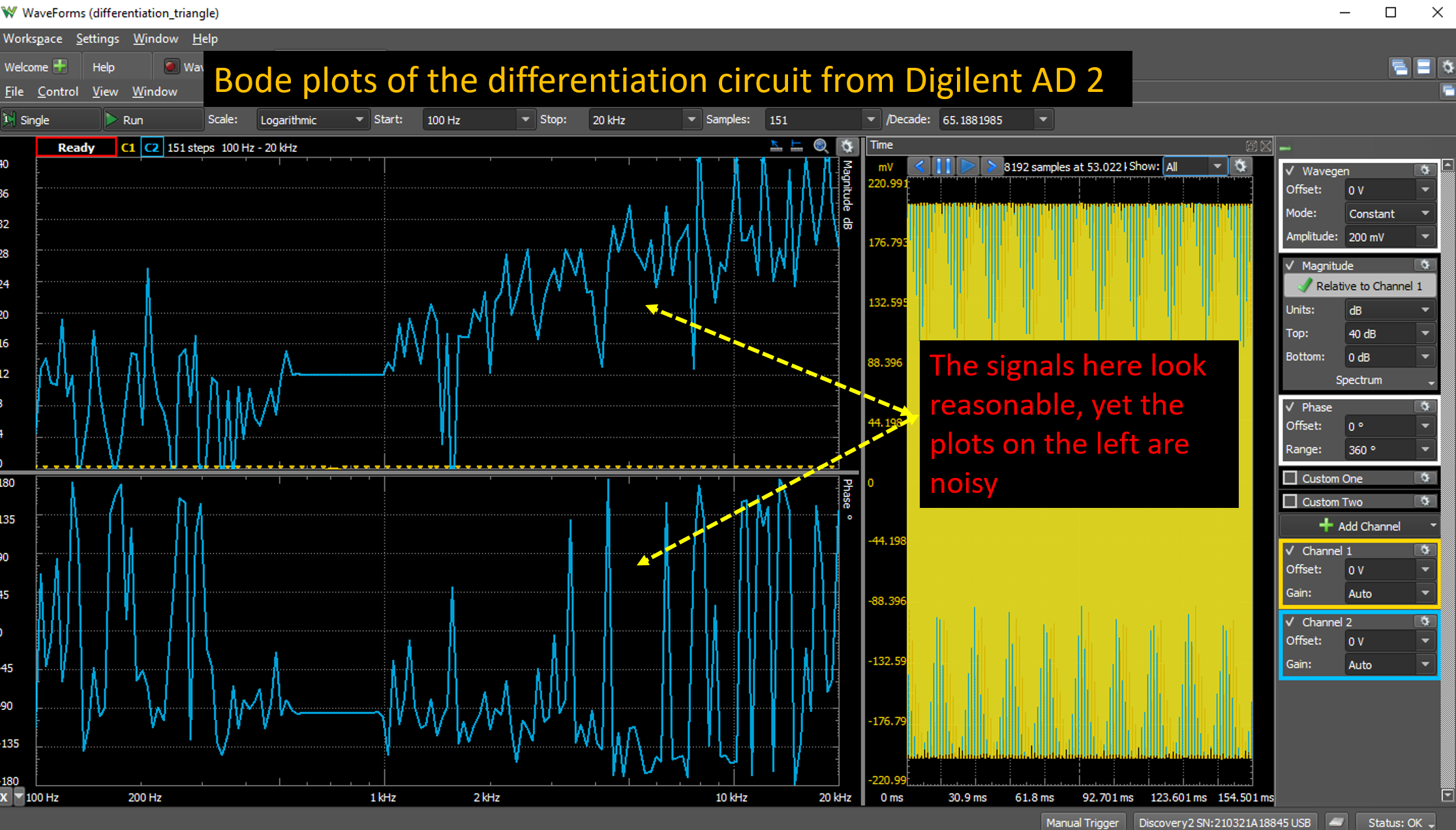
Here is what one should obtain:

Bode plots: the dots mark experimental data. The continuous curves are calculation from the circuit simulation app.
  
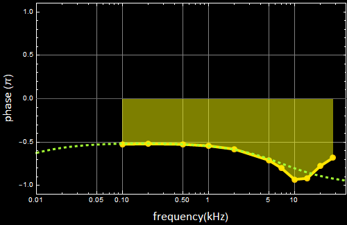
The model in the app does not include specific resonance of this particular op amp (741), which causes the deviation above 10 kHz (see below for an older-version circuit that includes this 741 op amp model).

If you choose to build the older version alternative differentiation circuit as shown below:

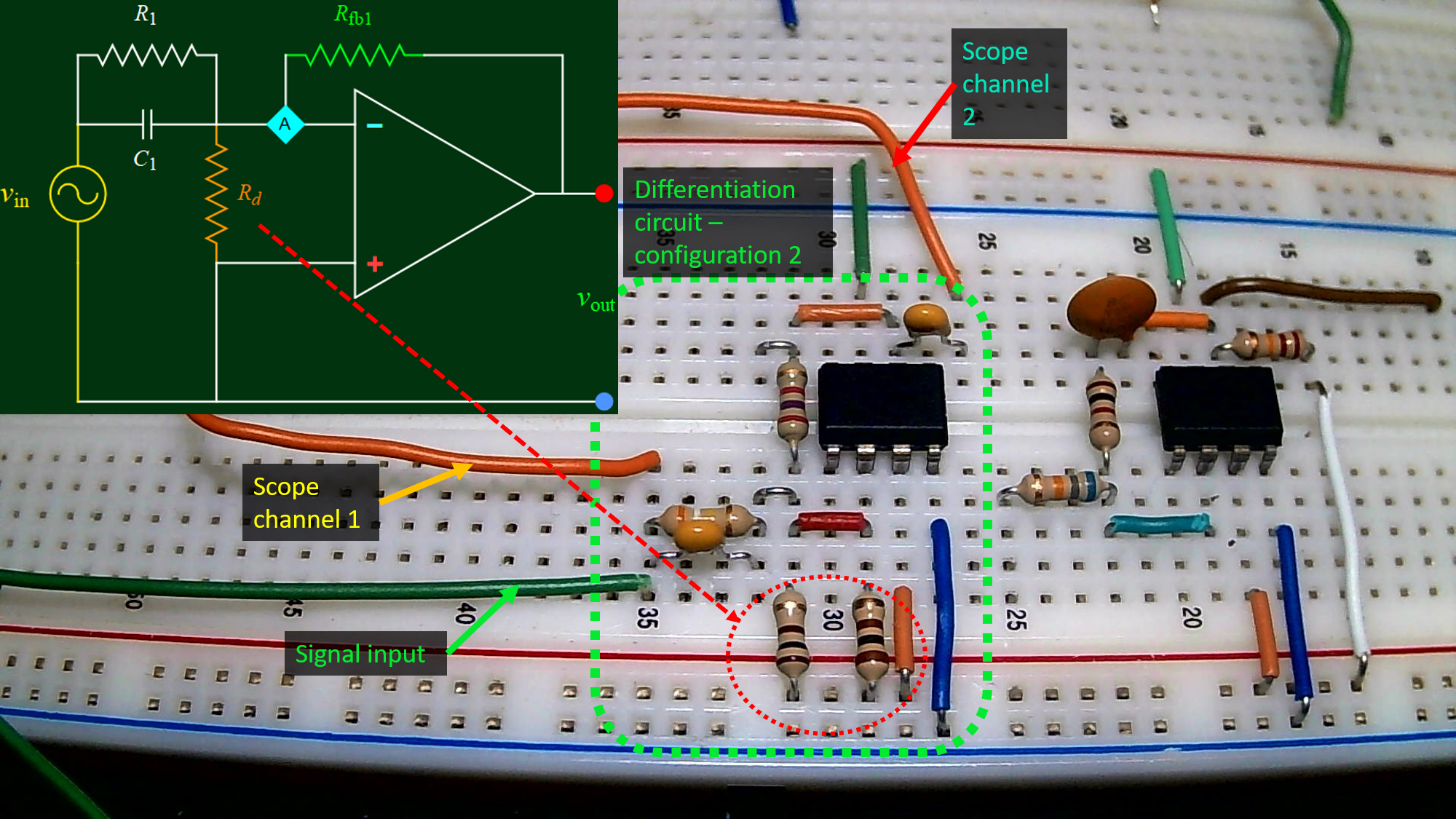
see the table for components on page 3: use serial or parallel technique to get closest C and R values you wish. For example, if you don't have non-electrolytic 0.1 uF, just use 0.047+0.033+0.022 (uF) in parallel.


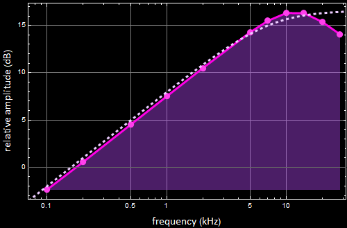
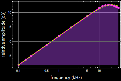
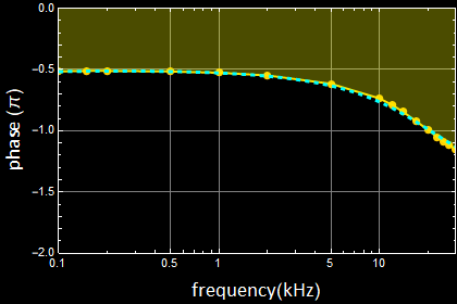
You should get the frequency response results like the below:


Bode plots for magnitude (left) and phase (right). The points and the solid curves are experimental results (the actual circuit in the picture above), the dashed curves are from the theoretical model (see the transfer function below).
  

Below are Nyquist plot 2D and 3D
    
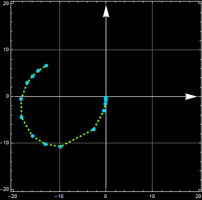
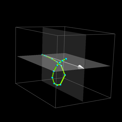
(go to the class note page or app page for the app producing the graphics above).

The only part that matters is the 1st-order circuit behavior portion between 0.1 and 10 kHz. You need not be concerned with the part related to this particular op amp behavior above 10 kHz.

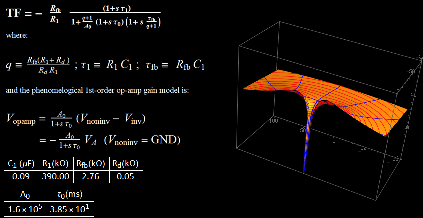
If you have learned Laplace-transformed circuit theory, below is the transfer function, FYI. Do not be concerned if you have not learned the topic.

3D plot of the transfer function.



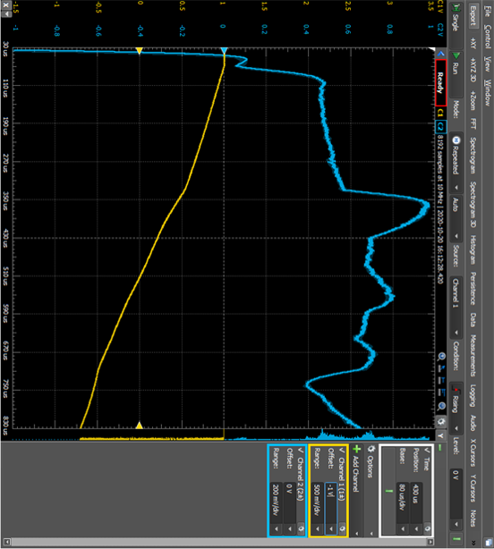
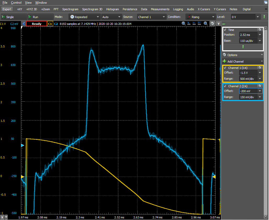
Step B.4: 

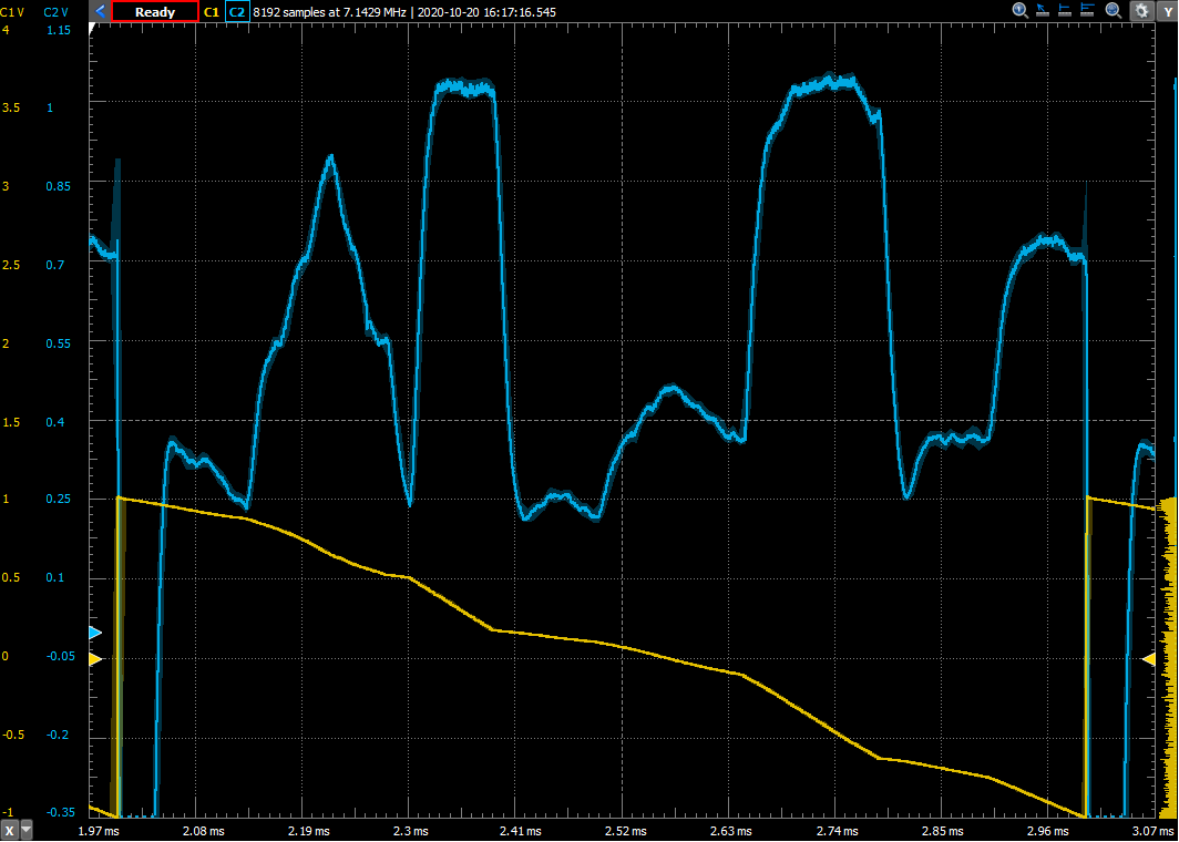
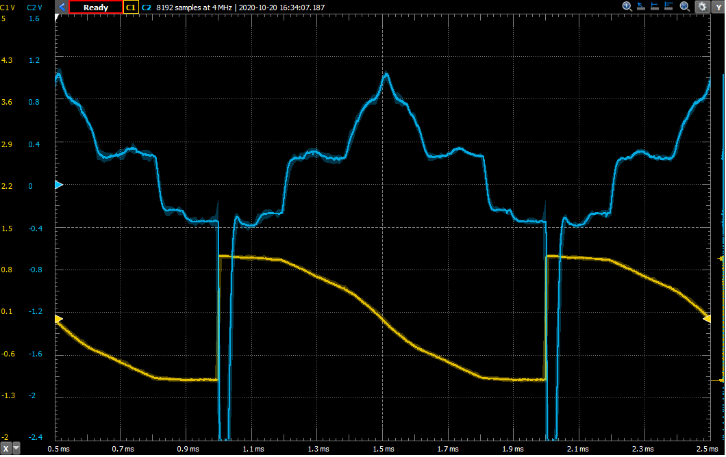
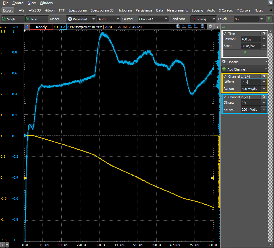
Step B.5: what are these waveforms? In the figures below, yellow is the input, blue is the output from the differentiation circuit.